Neutrino transport, unpacked: why it is so hard and what people do about it

The previous post set up the Boltzmann equation for radiation and listed, briefly, what changes when the radiation is neutrinos in a core-collapse supernova or a merger remnant. This post goes through those difficulties properly. The goal is that by the end you could look at any neutrino transport scheme and know which of these problems it is solving and which it is quietly ignoring.

For concreteness I'll keep talking about the core-collapse supernova: an iron core the size of the Earth collapses to a proto-neutron star thirty kilometres across in a quarter of a second, the shock that forms stalls at around 150 km, and the question is whether neutrino heating behind the shock will revive it. Everything below applies, with small changes, to neutron star mergers and to collapsar disks.

Counting the unknowns

Start with the phase space. The distribution function depends on three positions, one energy, two angles, and the species. A supernova simulation with a few hundred cells in each spatial direction is a modest one; energies between 1 and 300 MeV need a dozen or two logarithmically spaced groups; and the angular distribution needs enough directions to tell a forward-peaked beam from an isotropic bath. Here is how the number of unknowns per cell grows as you keep more of the phase space.

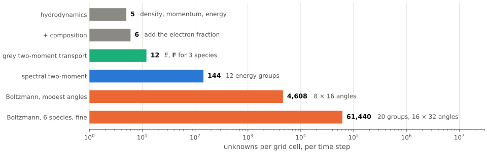
Horizontal bar chart on a log scale of unknowns per grid cell: 5 for hydrodynamics, 6 with composition, 12 for grey two-moment transport, 144 for spectral two-moment with 12 groups, 4,608 for Boltzmann with 12 groups and 8 by 16 angles, and 61,440 for 6 species with 20 groups and 16 by 32 angles. — Unknowns per grid cell for the gas and for various levels of neutrino transport. A three-dimensional grid of \(500^3\) cells carries \(1.25\times10^8\) cells, so the last row is \(8\times10^{12}\) numbers, about 60 terabytes per copy of the solution, and a time step has to touch every one of them.

The direct approach, keeping all the angles and energies on a 3D grid, has been done, but only in the last few years, only at low angular resolution, and only by groups with access to the largest machines in the world. It is a research project in itself, not a tool you run a parameter study with. Everyone else is throwing something away, and the first question to ask of a scheme is which dimensions did it drop.

The collision term is stiff

Dimensionality is the obvious cost. The less obvious one is time. The collision term in the Boltzmann equation drives the distribution toward equilibrium at a rate set by the interaction time, the mean free path divided by \(c\). Near the centre of the proto-neutron star that time is below a nanosecond. The hydrodynamic time step, set by the sound speed and the cell size, is about a microsecond. The ratio is \(10^4\) or more.

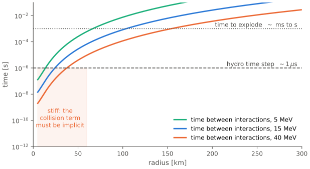
Time between interactions for neutrinos of three energies in the toy proto-neutron star from the previous post, compared with the hydrodynamic time step and the time over which the explosion develops. Inside the neutrinosphere the collision term acts thousands of times per hydro step.

An explicit scheme, one that computes the collision rates from the current state and adds them on, would need a time step shorter than the interaction time to be stable, so about \(10^4\) steps where the hydro takes one. The collision term has to be treated implicitly: solve for the state at the end of the step such that the rates evaluated there produce that state. That is a nonlinear equation, because the rates depend on the distribution through the Pauli blocking factors and because the matter temperature and composition respond to the energy and lepton number the neutrinos deposit. In practice every cell, every step, needs a Newton-Raphson solve on a system that couples all energy groups and all species, with the matter state as additional unknowns. In a moment scheme with 12 groups and 3 species that is a system of some 150 equations per cell. In a full Boltzmann scheme it is tens of thousands. The linear algebra inside that solve is where most of the time of a transport code goes.

Energies talk to each other

If a neutrino kept its energy from emission to absorption, the energy groups would be independent and the transport could be done one group at a time, like a set of grey problems. They are not independent. Scattering on electrons transfers a large fraction of the neutrino's energy to the electron. Scattering on nucleons, which is nearly elastic for a single event because the nucleon is so heavy, still shifts the energy by a percent or so per collision, and in the opaque region a neutrino collides thousands of times before it leaves. Those small shifts are what let heavy-lepton neutrinos, which cannot be absorbed, exchange energy with the matter at all, and getting them wrong changes the \(\nu_x\) spectrum by MeVs. Pair processes, the creation of a \(\nu\bar\nu\) pair from an electron-positron pair or from two nucleons scattering, couple a neutrino in one energy group to an antineutrino in another.

Left: neutrino cross sections versus energy on a log scale for absorption on neutrons, elastic scattering on neutrons, coherent scattering on iron nuclei, and inelastic scattering on electrons; the first three rise as energy squared. Right: three small matrices showing which energy groups are coupled by each process: only the diagonal for absorption and emission, a band around the diagonal for inelastic scattering, and the full matrix for pair processes. — Left: approximate cross sections of the main reactions (scaled from the standard low-energy formulas; order of magnitude only). Coherent scattering on heavy nuclei dominates during collapse, which is why the core traps its neutrinos and lepton number at all. Right: the coupling structure of the implicit solve. Absorption and emission act within an energy group; inelastic scattering couples neighbouring groups; pair processes couple everything to everything, including neutrinos to antineutrinos.

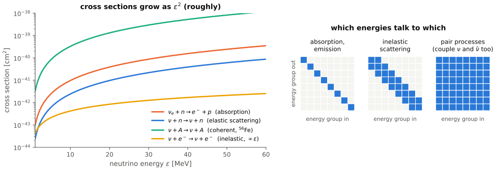
The structure on the right is the structure of the matrix in the implicit solve. With only emission and absorption it is diagonal in energy and trivially cheap. With inelastic scattering it is banded. With pair processes it is full, and a full matrix of size (groups \(\times\) species) per cell per step is the price of getting the \(\nu_x\) right.

There is a further problem hiding in the left panel. The rates themselves are not known to better than ten or twenty percent in the conditions that matter. The nucleons in the proto-neutron star are not free: they interact with each other, their effective masses change, and the medium screens the weak interaction in ways that depend on nuclear physics that is still being worked out. These are not academic corrections. Changing the neutral-current scattering opacity by about ten percent, within what nuclear physics allows, has turned models that failed to explode into models that did. So the transport has to be accurate enough that the remaining uncertainty is in the physics inputs and not in the numerics, which means better than ten percent in the heating rate.

Three regimes, one object

Then there is the problem from the previous post, now with numbers. For a 15 MeV neutrino in the toy proto-neutron star, the optical depth to infinity is a thousand at the centre, one at about 60 km, a tenth at 100 km and a hundredth at the shock.

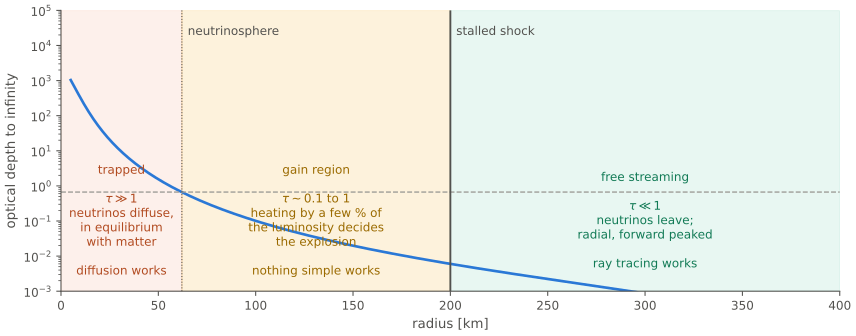
Optical depth to infinity versus radius for 15 MeV neutrinos, on a log scale, with three shaded regions: the trapped region inside 60 km where diffusion works, the gain region between the neutrinosphere and the stalled shock at 200 km where nothing simple works, and the free-streaming region outside the shock where ray tracing works. — The three transport regimes in a stalled-shock supernova core, for one neutrino energy. Each energy has its own neutrinosphere, so the boundaries smear over tens of kilometres. The region that decides the outcome is the one in the middle.

In the trapped region the neutrinos are in equilibrium with the matter and diffuse; a diffusion solver is right there. Outside the shock they stream radially and a ray tracer is right. The gain region between the neutrinosphere and the shock is where neither is right, and it is where the heating happens. The heating rate per nucleon is proportional to the local neutrino energy density times the mean squared energy, and both depend on how fast the radiation field makes the transition from isotropic to forward-peaked. If a scheme makes that transition too early, it moves energy out too fast and underestimates the energy density in the gain region; too late, and it overestimates it. Either way the error lands directly in the one number that matters.

A good transport scheme, then, is not one that is accurate in the thick limit and in the thin limit. Those are easy. It is one that is accurate in between, and that is what the test problems in the next post are designed to probe.

Everything moves

The matter behind the shock falls at \(0.1c\), the proto-neutron star contracts, and in a merger or a collapsar disk the orbital speeds are a third of light. The transfer equation in the lab frame has a simple left side (straight lines at \(c\)), but the collision term is simple only in the frame moving with the matter, where the opacities are isotropic functions of the local temperature and density. Translate between the two and you get the velocity-dependent terms: Doppler shifts of the energies, aberration of the directions, and a term that moves neutrinos between energy groups at a rate proportional to the velocity gradient.

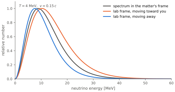
Three neutrino number spectra: a thermal spectrum at 4 MeV in the frame of the matter, and the same spectrum seen in the lab frame from matter moving toward the observer at 0.15c (shifted to higher energy) and away (shifted to lower energy). — A thermal spectrum emitted by matter moving at \(0.15\,c\), as seen in the frame of the matter and in the lab frame along and against the direction of motion. The mean energy shifts by about 15%, and because the absorption cross section goes as energy squared, the heating from that spectrum changes by 30% or more. Nothing in the problem is small enough to drop.

These terms are of order \(v/c\) and it is tempting to drop them. The lesson of the 2000s was that you cannot. Simulations that left them out got the energy and lepton-number budgets wrong by tens of percent, enough to change the outcome. In general relativity there is also the gravitational redshift, 20 to 30% at the surface of the proto-neutron star, and the bending of neutrino paths, which matters for how much of the neutrino flux from the far side of the star reaches the gain region on the near side. A modern code handles all of this consistently or it is not trusted.

The practical headache is that the energy-shift terms are derivatives in energy space, and discretizing them so that neutrino number and neutrino energy are both conserved is genuinely difficult. A scheme that conserves one and not the other will, over the many thousands of steps of a simulation, either create or destroy lepton number or energy out of nothing. Several papers from around 2010 are devoted entirely to this one discretization.

Nothing is allowed to leak

Which brings up conservation in general. The neutrinos carry away about \(3\times10^{53}\) erg, and the explosion has about \(10^{51}\) erg. A leak of one percent of the neutrino energy, in the wrong place, is an explosion's worth of energy. The energy the neutrinos lose must be exactly what the matter gains, the momentum likewise, and the electron-lepton number, which sets whether the ejecta end up neutron-rich or proton-rich and therefore what elements they make, must be tracked to a fraction of a percent. Operator splitting, where the hydro step and the transport step are done one after the other, has to be arranged so that the exchange terms are evaluated once and applied with opposite signs to both sides. This is the same discipline as refluxing in an AMR code, applied to a coupling instead of to a grid interface.

And it has to be three-dimensional

Finally, the problem is not spherical. The gain region is convective, the shock sloshes and spirals, the proto-neutron star itself convects, and whether the explosion happens depends on the multi-dimensional flow. The transport has to be multi-dimensional too, or at least not get in the way. The cheap compromise, solving a separate one-dimensional transport problem along each radial ray, loses the sideways exchange of neutrinos between hot and cold columns, and overstates the contrast between them. Doing the lateral transport properly multiplies the cost of a scheme several times over, and whether the compromise is acceptable is still argued about.

What people do

Here is the landscape. The columns are the parts of the problem described above; the bar is a rough cost relative to the hydrodynamics alone.

A matrix of eight transport methods (leakage, light bulb, flux-limited diffusion, IDSA, M1 two-moment, variable Eddington factor two-moment, discrete ordinates, Monte Carlo) against five aspects of the problem (energy spectrum, angular distribution, time dependence, lateral transport, velocity and GR terms), with filled, half-filled or empty circles, and a bar for the relative cost rising from about 1 to about 5000 times the hydro. — What each approach keeps. The circles are a judgment, not a measurement: a half circle means the method includes the effect in some reduced form, and the details differ between implementations. Costs are order of magnitude and depend heavily on the number of energy groups and on how the implicit solve is done.

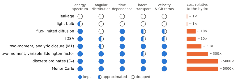
Reading from the top:

Leakage schemes don't transport anything. In each cell they estimate how quickly neutrinos would be produced locally and how long it would take them to diffuse out, combine the two into an effective loss rate, and remove that much energy and lepton number from the matter. There is no radiation field, so no heating unless it is added by hand. Cost: nothing. Used in merger simulations and in the first three-dimensional supernova studies, and still used when the point of the simulation is something other than the transport.

Light-bulb schemes go the other way: they assume a neutrino luminosity and spectrum coming from the centre and compute the heating from it with a simple absorption law. The transport is replaced by a parameter, which is exactly what you want if the question is "how much heating does it take to explode this star?"

Flux-limited diffusion (FLD) solves the diffusion equation for the energy density in each group, with a factor that caps the flux at \(cE\) so that the solution does not move faster than light in the transparent region. It is a one-moment method: it has an energy density but no independent flux, so the radiation has no memory of its direction, and it cannot cast a shadow or keep a beam together. The workhorse of supernova modelling through the 2000s, usually in the ray-by-ray form.

IDSA, the isotropic diffusion source approximation, splits the distribution into a trapped part that is treated by diffusion and a streaming part that is treated by ray tracing, with a source term moving neutrinos from the first to the second. Cheap, and cleverer than FLD in the transition region, with the same lack of angular information.

Two-moment schemes evolve both the energy density and the flux, and close the system with a prescription for the pressure tensor. With an analytic closure (the M1 scheme, after the first moment) the pressure is a formula in terms of \(E\) and \(\mathbf{F}\), chosen to be right in the diffusion and free-streaming limits and to interpolate smoothly in between. The radiation can now stream in a direction and cast a shadow. This is the most common choice in current multi-dimensional codes. Its known failure is that it treats the radiation at a point as a single beam, so two beams crossing are merged into one.

With a variable Eddington factor closure, the pressure tensor is instead taken from a cheap, simplified solution of the Boltzmann equation itself, usually in one dimension, iterated to consistency. More accurate, several times the cost, and the approach of the Garching group's Vertex code, which has been the reference for one- and two-dimensional supernova modelling for twenty years.

Discrete ordinates (\(S_N\)) solves the Boltzmann equation directly on a grid in angle as well as space. Everything is kept. The cost is the full phase space, and the characteristic artefact is the ray effect: with a finite set of directions, radiation from a small source reaches only the cells that lie along those directions, giving a star-shaped pattern instead of a smooth one.

Monte Carlo samples the distribution with particles: emit packets at the local rate, move them in straight lines, draw their interactions from the cross sections. Also everything kept, with no angular grid and therefore no ray effects, and with a cost that scales gently with dimension. The price is statistical noise, which falls only as the square root of the number of packets, and the difficulty of doing the implicit collision term in the opaque region, where a packet would scatter millions of times per step. Modern Monte Carlo transport codes switch to diffusion for packets deep inside the opaque region to get around that. This is the approach taken in the code I work with, νbhlight, where the Monte Carlo packets live on the same grid as the general-relativistic magnetohydrodynamics and exchange energy and momentum with it every step.

Two further ideas cut across the table. Ray-by-ray means doing the transport in one dimension along each radial direction independently; it can be combined with any of FLD, IDSA, two-moment or variable Eddington factor methods, and it is how most of the two- and three-dimensional supernova simulations of the last fifteen years were done. And grey versus spectral (or energy-dependent, or multigroup) applies to everything: a grey scheme integrates over energy and carries one number where a spectral scheme carries one per group. Given the \(\varepsilon^2\) cross sections, grey neutrino transport is used only when nothing better is affordable, and some of the cleverest recent work is on making a grey scheme behave as though it were spectral by evolving the mean energy alongside the energy density.

The short version

Neutrino transport is hard because the problem is seven-dimensional, the collision term is stiff and nonlinear and couples every energy and species, the answer is decided in the regime where neither diffusion nor streaming is right, the matter moves at a good fraction of \(c\) in strong gravity, and nothing may leak. Every scheme in use is a decision about which of these to do properly. The next post takes the main ones in turn and, with small numerical experiments, shows what each one gets right and exactly where it breaks.