Neutrino transport approximations, one by one

The previous post ended with a table of neutrino transport methods and a promise to go through them properly. This is that post. For each method I'll give the idea, the equations in their simplest form, what it gets right, and the situation where it goes wrong. Wherever a failure can be shown in a picture, there is a picture, made with a two-dimensional toy solver that you can download and run. It has a two-moment solver, a flux-limited diffusion solver, and discrete-ordinates and Monte Carlo solutions for a point source, in about 200 lines of numpy and scipy.

The test problems are deliberately stripped down: a unit square, the speed of light set to one, a beam entering from the left, sometimes an opaque disc in the way. They have nothing to do with supernovae and that is the point. A method that cannot cast a shadow on a unit square cannot do it in a star either, and the failure is much easier to see without the hydrodynamics on top.

The methods are in rough order of increasing cost. If you only want the summary, it is the table at the end.

Leakage: no transport at all

The cheapest thing you can do is not transport neutrinos. A leakage scheme looks at each cell of the gas and asks two questions: how fast would this matter emit neutrinos if they could all escape, and how long would it take a neutrino produced here to diffuse out? The first gives a local emission rate $Q_\mathrm{loc}$, computed from the local temperature and composition with the same weak-interaction rates a real transport code uses. The second gives a diffusion time $t_\mathrm{diff} \sim 3\tau^2 \lambda / c$ (the random-walk time to cover $\tau$ mean free paths), compared to the local emission time $t_\mathrm{loc}$, the time it would take to build up the equilibrium neutrino density at the local rate. The two are combined into an effective loss rate:

$$ Q_\mathrm{eff} = \frac{Q_\mathrm{loc}}{1 + t_\mathrm{diff}/t_\mathrm{loc}} . $$

Where the matter is transparent, $t_\mathrm{diff}$ is short and the neutrinos leave at the local rate. Where it is opaque, the loss is throttled to what diffusion allows, $Q_\mathrm{eff} \approx e_\mathrm{eq} / t_\mathrm{diff}$, which no longer depends on how fast the matter can emit. That energy and the corresponding lepton number are removed from the cell, and that is all.

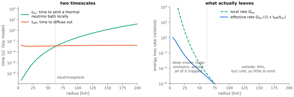
Leakage in the toy proto-neutron star from the earlier posts. Left: inside the neutrinosphere a cell would emit a thermal bath of neutrinos in microseconds but needs milliseconds to get rid of it; outside, the opposite. Right: the effective rate is the local rate, throttled by the ratio of the two. Deep inside it is suppressed by orders of magnitude.

The formula above is from Ruffert, Janka and Schäfer (1996), who used it for neutron star mergers, and it was adapted to supernova cores by Rosswog and Liebendörfer (2003) and later put into general relativity by O'Connor and Ott (2010). The optical depth $\tau$ is the only non-local input, and it is computed by integrating the opacity outward along rays, so even that is cheap.

What it gets right is surprising. The total neutrino luminosity comes out within a factor of two of a real transport calculation, the deleptonization of the core during collapse is roughly right, and the cooling of a merger remnant is right enough to follow its evolution for tens of milliseconds. What it misses is everything that requires knowing the radiation field. There is no energy density anywhere, so there is no heating: the gain region does not exist. Schemes that add a heating term by hand, from the leakage luminosity and an assumed spectrum, exist (the "advanced spectral leakage" of Perego and collaborators, 2016, is the most careful), and they turn leakage into something like a self-consistent light bulb. There is no spectrum, so the composition of the ejecta, which depends on the difference between the $\nu_e$ and $\bar\nu_e$ mean energies, is a guess.

Leakage is the right tool when the neutrinos are a sink and nothing else: the first milliseconds of a merger, a survey over many progenitors where the question is the collapse dynamics and not the explosion, or any simulation in which the transport is not the point and cannot be afforded.

Light bulb: assume the answer

The opposite simplification. A light-bulb scheme does not compute what the proto-neutron star emits; it assumes it. You fix a luminosity $L_\nu$ and a spectrum (a temperature $T_\nu$) for each species, and the heating at radius $r$ is simply what that luminosity would deposit if it streamed radially out from the centre:

$$ \mathcal{H} \propto \frac{L_\nu}{4\pi r^2}\, \langle\varepsilon_\nu^2\rangle\, e^{-\tau} , $$

with a cooling term $\propto T^6$ for the matter's own emission. The $\varepsilon^2$ is the cross section, the $e^{-\tau}$ switches the heating off inside the neutrinosphere, and $T^6$ is the temperature dependence of electron and positron capture on nucleons.

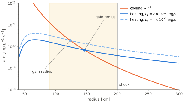
Heating and cooling rates versus radius on a log scale for two assumed neutrino luminosities. The cooling curve falls steeply with radius; the heating curves fall as one over r squared. They cross at the gain radius, which moves inward when the luminosity is doubled. — Light-bulb heating and cooling in a toy post-shock profile. The gain radius, where heating overtakes cooling, is where the gain region begins; above it, matter gains energy from the neutrinos until it is swept through the shock. Doubling the luminosity moves the gain radius in and makes the gain region deeper.

This gives up any claim to predict whether a given star explodes. What it gives in return is a clean experiment: with the neutrino luminosity as a dial, you can ask how much heating a given stalled shock needs to be pushed out, and how that threshold depends on things like dimensionality, rotation, or the progenitor. Burrows and Goshy (1993) turned this into the idea of a critical luminosity curve, and most of what we learned in the 2000s about why multi-dimensional supernovae explode more easily than spherical ones came from light-bulb simulations in which everything else was held fixed. The approach is still used for exactly that purpose.

The failure mode is not numerical. It is that the neutrino emission is not independent of the flow: the accretion onto the proto-neutron star powers a large part of the luminosity, and when the shock expands and accretion drops, so does the luminosity. A light bulb cannot see that feedback, and so it tends to explode too easily.

Flux-limited diffusion: one moment

Now we actually transport something. The first moment equation from the first post is a conservation law for the energy density, with the flux as its unknown:

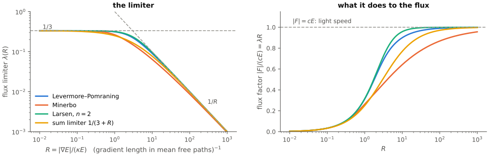
$$ \frac{\partial E}{\partial t} + \nabla\cdot\mathbf{F} = \text{sources} . $$

In the opaque limit we know the flux: $\mathbf{F} = -(c/3\kappa)\nabla E$. Put that in and you have a diffusion equation for $E$, one unknown per cell per energy group, which can be solved implicitly for any time step. The problem is the transparent region, where the diffusion formula gives a flux that grows without bound as $\kappa \to 0$, faster than the speed of light. Flux-limited diffusion keeps the diffusion form but inserts a factor that caps the flux:

$$ \mathbf{F} = -\frac{c\,\lambda(R)}{\kappa}\nabla E, \qquad R = \frac{|\nabla E|}{\kappa E} . $$

$R$ measures how steep the energy density gradient is compared to the mean free path. When $R \ll 1$ the gradient is gentle on the scale of a mean free path and we are in the diffusion regime, so $\lambda \to 1/3$. When $R \gg 1$ we are in free streaming and $\lambda \to 1/R$, which makes $|\mathbf{F}| = cE$ regardless of the opacity. Several functions do this interpolation; the one from Levermore and Pomraning (1981) is derived from a model of the angular distribution, the Minerbo one from maximum entropy, and the "sum" limiter $1/(3+R)$ is just the simplest thing with the right limits.

Left: four flux limiter functions on log-log axes versus R, all equal to 1/3 at small R and 1/R at large R, differing by up to a factor of two near R of 1 to 10. Right: the resulting flux factor, rising from 0 to 1 as R goes from 0.1 to 100. — Flux limiters. They agree in both limits by construction; they differ in the transition, which is where the answer is decided. The Minerbo limiter approaches the light-speed limit most slowly.

Flux-limited diffusion, with energy groups and usually in the ray-by-ray form described below, was the standard in supernova simulations from the 1980s to about 2010: Bruenn's multigroup FLD, the Oak Ridge group's CHIMERA code, Burrows' early two-dimensional work. For the opaque core it is correct, and it is cheap enough to afford many energy groups.

Its problem is structural. There is one unknown per cell, the energy density, and the flux is defined to point down the gradient of $E$. The radiation has no memory of which way it was going. In the transparent region that produces behaviour that is simply wrong, and the standard way to see it is the shadow test: shine a beam at an opaque obstacle and look behind it.

Three panels showing radiation energy density on the unit square with a beam entering from the left and an opaque disc in its path. Exact: a sharp beam with a sharp shadow behind the disc. Flux-limited diffusion: the radiation spreads over the whole square and fills in behind the disc; no shadow. Two-moment M1: the beam stays together and the shadow behind the disc is dark. — The shadow test. A beam of width 0.4 enters from the left with a weak background absorption (optical depth 0.3 across the box) and hits an opaque disc. Exact: the geometric shadow. Flux-limited diffusion: the beam spreads in every direction as soon as it enters, because the flux follows the gradient of $E$ and at the edge of the beam that gradient points sideways; the shadow is lit to about a tenth of the beam's brightness. Two-moment: the beam holds together (with some smearing from the numerics) and the shadow is dark, with a leak of under 1%.

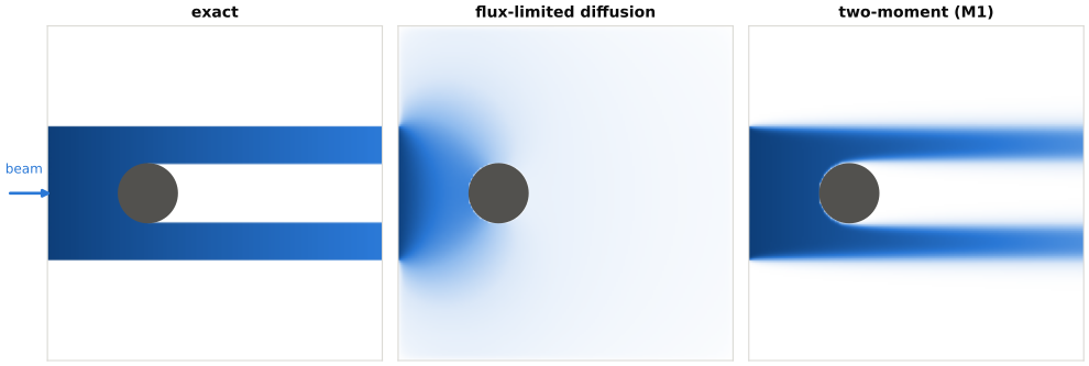
In a supernova, FLD's inability to keep a direction means it cannot represent the forward-peaked radiation field above the neutrinosphere, where the flux factor should rise toward one. It tends to keep the energy density too isotropic (too much $E$ for a given flux) in the gain region, which overestimates the heating there, and it leaks radiation sideways between hot and cold regions that should not be communicating. Most codes that used FLD have moved on. For photon transport in problems that are mostly opaque, like the interior of a star-forming cloud, it is still a reasonable choice.

Two-moment schemes: energy and flux

The fix is obvious once you see the problem: carry the flux as an independent unknown. Keep both moment equations,

$$ \frac{\partial E}{\partial t} + \nabla\cdot\mathbf{F} = \text{sources}, \qquad \frac{1}{c^2}\frac{\partial\mathbf{F}}{\partial t} + \nabla\cdot\mathsf{P} = -\frac{\kappa}{c}\mathbf{F} , $$

and close them with a prescription for the pressure tensor $\mathsf{P}$. Four unknowns per cell per group in 3D instead of one, and a hyperbolic system (signals move at finite speed, at most $c$) instead of a parabolic one, which means the methods from the upwinding post apply directly: Riemann solvers, limited reconstruction, the lot. Radiation now has a direction and keeps it.

The closure is where the physics is. Write $\mathsf{P} = \mathsf{D}E$ with the Eddington tensor

$$ \mathsf{D} = \frac{1-\chi}{2}\,\mathsf{I} + \frac{3\chi - 1}{2}\,\hat{\mathbf{n}}\hat{\mathbf{n}}, \qquad \hat{\mathbf{n}} = \frac{\mathbf{F}}{|\mathbf{F}|} , $$

which is isotropic when the Eddington factor $\chi = 1/3$ and is a pure beam along the flux when $\chi = 1$. The closure is then a single function $\chi(f)$ of the flux factor $f = |\mathbf{F}|/cE$. The one in nearly every neutrino code is Levermore's (1984):

$$ \chi(f) = \frac{3 + 4f^2}{5 + 2\sqrt{4 - 3f^2}} , $$

which is what you get if the radiation is isotropic in some frame moving at speed $f$ relative to the matter. Minerbo's (1978) closure comes instead from the angular distribution with maximum entropy for a given $E$ and $\mathbf{F}$. They differ by a few percent at intermediate $f$. This family of methods is usually called M1, for "first moment".

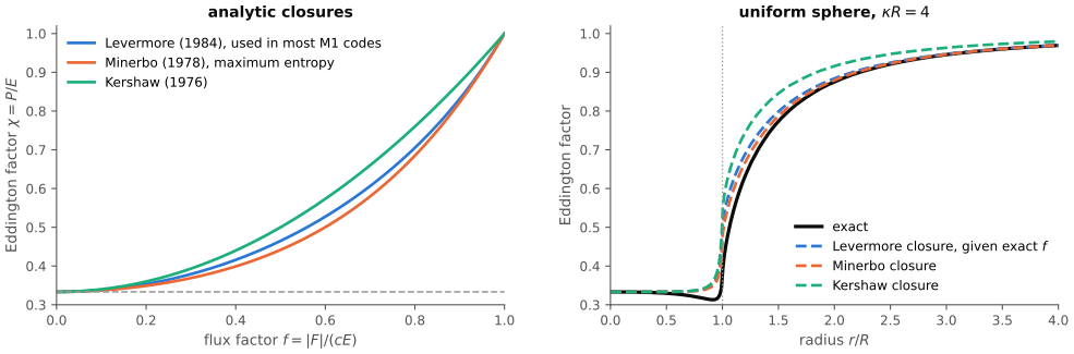
Analytic closures, and how they do on the uniform sphere from the first post ($\kappa R = 4$). Even given the exact flux factor, the closures overestimate the Eddington factor just outside the surface, where the radiation is a wide cone rather than the narrow beam or isotropic bath the closure interpolates between. Maximum error 0.12 for Levermore, 0.09 for Minerbo, 0.16 for Kershaw.

The uniform sphere test shows the kind of error a closure makes: the real radiation field outside an extended source is a cone of a definite opening angle, and no single function of $f$ can represent a cone. The closure gets the limits right and interpolates in between, and the error of order 0.1 in $\chi$ near the surface is the price. In a supernova this error sits exactly at the neutrinosphere, and comparisons against Boltzmann solutions find that M1 gets the heating in the gain region right to within about 10%, with errors of that order in the flux factor in the transition.

The second, more famous failure is in the picture below. Since the closure uses only $E$ and $\mathbf{F}$ at a point, it cannot tell the difference between one beam going right and two beams crossing at an angle. It sees their sum: a flux pointing right with a flux factor below one, which the closure interprets as a single, partly isotropic beam.

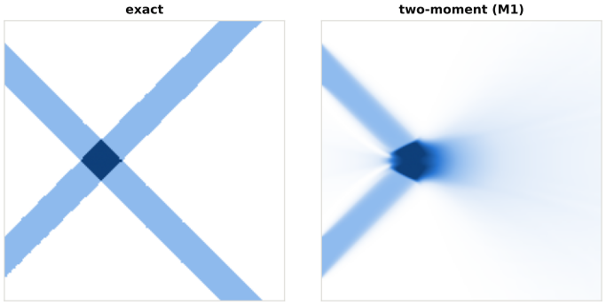
Two panels. Exact: two diagonal beams cross in the middle of the unit square and continue to the opposite corners. M1: the beams approach, merge where they meet into a bright blob, and leave as a single smeared beam going right, with faint remnants in the original directions. — Two beams crossing in vacuum. Exact: they pass through each other. M1: they collide. The closure has no way to represent two directions at one point, so where the beams overlap it produces a single flux pointing between them, and that is where the radiation goes.

Where does this matter? Anywhere radiation from different sources meets. Above a merger remnant or a collapsar disk, neutrinos from the two faces of the disk converge toward the rotation axis, and M1 schemes are known to produce a spurious bright column of radiation along the axis there, which is a real concern for the composition of the polar outflow. In the supernova gain region the problem is milder, because the radiation comes from one extended source, but the slight convergence of rays from different parts of the neutrinosphere is still misrepresented.

Despite this, two-moment with an analytic closure is the choice of most current three-dimensional supernova and merger codes: FORNAX, ALCAR, FLASH-M1, the Zelmani and GR1D codes, Kuroda's full-GR code, and others. It keeps the direction, it is a hyperbolic system that can be solved with standard tools, the energy groups can be treated with the full velocity-dependent terms, and the cost is modest: a dozen groups times three species times four unknowns, with an implicit solve for the source terms that is nonlinear but local to each cell.

Variable Eddington factor

If the closure is the weak point, compute it. The variable Eddington factor method keeps the two-moment system for the actual transport but takes $\chi$ from a cheap solution of the Boltzmann equation for the same problem, usually with simplified physics or in reduced geometry, and iterates the two to consistency. The moment equations enforce conservation and handle the stiff source terms; the Boltzmann solve provides the angular information they lack. This is the approach of the Vertex code of the Garching group (Rampp and Janka, 2002), which solves the angular problem along tangent rays in spherical symmetry and has been the reference solution for one- and two-dimensional supernova modelling for two decades. The cost is several times M1, and in multi-dimensional use it has been applied ray-by-ray.

Ray-by-ray and IDSA

Two more ideas that cut across the methods above.

Ray-by-ray means doing the transport in one dimension along each radial direction of the grid, independently, with the lateral components of the flux set to zero. In a spherical grid with 100 angular directions you run 100 one-dimensional problems. Each is cheap and parallel, and the one-dimensional solver can be as sophisticated as you like (Vertex's variable Eddington factor, in the Garching 2D and 3D runs; CHIMERA's multigroup FLD). This is how most multi-dimensional supernova simulations of the 2000s and 2010s were done.

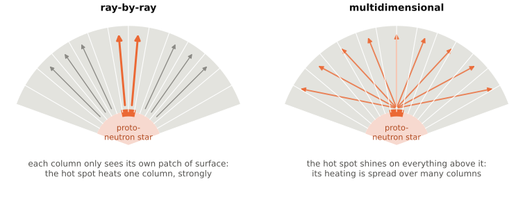
What ray-by-ray leaves out. A hot patch on the neutrinosphere actually shines on everything above it; in ray-by-ray it heats only its own column, and more strongly. Convection in the proto-neutron star makes such patches all the time.

The problem is in the figure. The neutrinosphere is not uniform: it is convective, and hot and cold patches on it come and go. Radiation from a hot patch really spreads over a wide angle, so by the time it reaches the gain region its heating is smeared over many columns. In ray-by-ray it stays in its column, and the heating above a hot patch is overestimated while the heating above a cold patch is underestimated. Since the explosion depends on the strongest heating anywhere, this bias is in the direction of making explosions easier, and whether it is large enough to matter was debated vigorously in the 2010s. The comparisons that have been done (Skinner, Burrows and Dolence, 2016; Glas and collaborators, 2019) found differences in the explosion time and energy that are not negligible but not decisive. Codes written since then mostly do the full multi-dimensional transport.

IDSA, the isotropic diffusion source approximation of Liebendörfer, Whitehouse and Fischer (2009), is a different kind of split. The distribution function is written as a trapped part plus a streaming part. The trapped part is treated by diffusion with the local matter and is isotropic by assumption; the streaming part is computed by integrating the emission of the trapped part outward along rays, which is cheap. A source term converts trapped neutrinos into streaming ones at a rate set by the local diffusion time. It is a cleverer version of leakage in which the leaked neutrinos are then followed, and it is cheap enough to be used in three dimensions with many energy groups. Its limitations are those of its pieces: the streaming part is radial, so it is a ray-by-ray method, and heavy-lepton neutrinos are usually handled by leakage.

Boltzmann solvers

Everything so far is a model of the angular distribution. The last two methods solve for it.

Discrete ordinates

Put a grid on the directions. Choose $N$ unit vectors $\mathbf{n}_k$ with weights $w_k$, write one transfer equation per direction,

$$ \frac{1}{c}\frac{\partial I_k}{\partial t} + \mathbf{n}_k\cdot\nabla I_k = \eta - \kappa I_k + \kappa_s \sum_j w_j I_j , $$

and solve them as $N$ coupled advection equations. The scattering term couples the directions, and the pair processes couple the energies and species, so the implicit solve is over the whole phase space of a cell. This is the $S_N$ method of neutron transport, and it is what the one-dimensional Boltzmann solvers for supernovae used from the 1990s on (Mezzacappa and Bruenn's solver, Liebendörfer's AGILE-BOLTZTRAN). In three dimensions it has been done by Sumiyoshi and Yamada (2012) and by Nagakura and collaborators (2018 onward), with angular grids of a few dozen directions, and those remain among the most expensive supernova simulations ever run.

The characteristic error of a direction grid is the ray effect. A small source illuminates only the directions in the set, and a detector far away sees it only if it happens to lie along one of them.

Four panels of radiation energy density around a small source in vacuum, on a log colour scale. Discrete ordinates with 8 directions: eight bright spokes and darkness between them. With 32 directions: 32 spokes, still with dark gaps far from the source. Monte Carlo with 20,000 packets: a smooth fall-off with grainy noise, slightly streaky far from the source. Reference: a smooth one-over-r fall-off. — A small isotropic source in two-dimensional vacuum. The line integrals along each direction are done exactly, so the only error in the first two panels is the angular grid. With 8 directions the solution is nonsense a few source widths away; with 32 it is still wrong by 40% (rms) at a distance of twenty source widths. The Monte Carlo solution with 20,000 packets has no preferred directions and a 13% noise at the same distance, which drops to 4.5% with ten times as many packets.

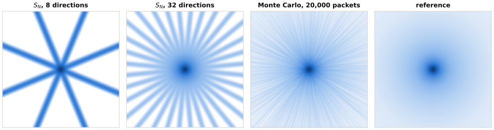
Ray effects are worst in the free-streaming region, where there is no scattering to redistribute radiation between directions, and for small sources. In a supernova the source is the whole neutrinosphere and the distances are a few source radii, which is the benign case, and a few dozen directions are enough for the heating rate. For a merger disk seen from the axis, or for any problem with a compact bright spot, they are not.

Monte Carlo

Instead of a grid in angle, sample. Emit packets of neutrinos at the local rate with random directions and energies drawn from the emissivity, move each one in a straight line, draw the distance to its next interaction from an exponential with the local mean free path, and at the interaction either absorb it (deposit its energy and lepton number in the gas) or scatter it (draw a new direction and energy). Tally the energy density and the heating from the paths. That is the whole method. There is no angular grid and no energy grid, so there are no ray effects and no numerical diffusion in angle or energy; the velocity and gravitational terms are handled by transforming each packet exactly; and adding a dimension does not change the algorithm at all.

The cost is noise. The tally in a cell is a sum over the packets that crossed it, and with $N$ of them the relative error is $1/\sqrt{N}$. Ten times the accuracy costs a hundred times the packets. The heating rate in the gain region needs to be known to a few percent in every cell, every step, which means thousands of packets per cell, and a modern supernova grid has millions of cells. The figure above shows the trade: a Monte Carlo solution has no systematic error and a random error that falls slowly.

The other difficulty is the opaque region. A packet deep inside the proto-neutron star scatters every few centimetres, so following it through a hydro time step means millions of scatterings per packet, all of which cancel to a tiny net drift. The standard fixes are to treat scattering in a cell as diffusion when the cell is many mean free paths thick (a random walk or discrete diffusion step moves the packet to the cell boundary in one go), and to treat absorption-emission implicitly (Fleck and Cummings' implicit Monte Carlo, 1971) by converting a fraction of absorptions into effective scatterings so that the stiff coupling with the gas does not need tiny time steps.

Monte Carlo neutrino transport was used first as a reference for one-dimensional problems (Janka in the early 1990s, Abdikamalov and collaborators in 2012, Richers' Sedonu code), and it is now being coupled to the dynamics: Foucart's merger simulations use it to calibrate an M1 scheme, and in the νbhlight code that I use for collapsar disks the packets move on the same grid as the general-relativistic magnetohydrodynamics, interacting with it every step. The number of packets is set by the computational budget, the noise is what it is, and the noise is at least random rather than biased.

Energy groups, and a word on grey transport

All of the transport methods above come in grey and spectral versions. Grey means integrated over energy: one $E$ and one $\mathbf{F}$ per species, with the energy dependence of the opacities replaced by averages over an assumed spectrum. Spectral (multigroup, energy-dependent) means one set per energy bin. For neutrinos, where the cross sections go as $\varepsilon^2$ and the decoupling radius depends on energy, the spectral version is the real thing and the grey version is a model of it: a grey scheme has to guess the mean energy of the neutrinos at every point to get the heating right, and getting that guess right near the neutrinosphere is most of the difficulty.

Spectral schemes have their own headache, the energy advection term from the Doppler and gravitational shifts, which moves neutrinos between groups and must be discretized to conserve number and energy at once. But once that is done, a spectral two-moment scheme with a dozen groups is the current standard, and the cost of the groups is linear.

Summary

Method	Keeps	Cost	Breaks when
Leakage	local cooling and deleptonization	nothing	you need heating, spectra, or the radiation field at all
Light bulb	a tunable heating profile	nothing	the luminosity should respond to the flow
Flux-limited diffusion	energy density and spectrum; diffusion limit exactly	low	the radiation needs a direction: beams, shadows, the transition region
Two-moment, M1	energy, flux, spectrum; both limits	moderate	beams cross or converge; cones from extended sources
Variable Eddington factor	the above with a computed closure	moderate to high	the reduced Boltzmann solve does not fit the geometry
Ray-by-ray (any of the above)	1D accuracy along each ray	as the 1D method	the neutrinosphere is not uniform
IDSA	a trapped-plus-streaming split	low	the streaming part needs to be non-radial
Discrete ordinates	the full angular distribution	very high	sources are compact: ray effects
Monte Carlo	the full distribution, no grid artefacts	very high, scales with packets	the tally must be smooth: noise falls only as 1/√N

None of these is the right answer. The right answer is the Boltzmann equation, and every entry is a position on the line between what it costs and what it leaves out. The honest thing a simulation can do is to say which position it took, and to have checked, on problems like the ones in this post, that the thing left out does not decide the result.

Try it

The script that made the shadow, crossing-beam and point-source figures runs in under a minute. Things worth doing with it: change the closure in the M1 solver to Minerbo's and rerun the crossing beams (the merge is still there; it is not the closure function's fault but the closure's existence). Replace the Levermore–Pomraning limiter with the sum limiter and watch the FLD shadow get worse. Put a second, weaker source in the point-source problem and see how many directions the discrete-ordinates solution needs before it can see it. Give the Monte Carlo solution a scattering opacity and watch the run time grow with it.