Upwinding and reconstruction in astrophysical fluid codes

In the last post I said that most astrophysical fluid codes are shock-capturing finite-volume codes, and I moved on quickly. This post looks inside one. Two ingredients do almost all of the work, and there is a long list of named variants of each: upwinding, which decides which way information flows, and reconstruction, which decides how much detail you can recover from a grid of averages. If you've ever read a simulation paper with a sentence like "we use PPM reconstruction and the HLLC Riemann solver", this is what that sentence means.

The simplest equation that goes wrong

Strip fluid dynamics down as far as it will go and you get the advection equation:

$$ \frac{\partial u}{\partial t} + a\,\frac{\partial u}{\partial x} = 0. $$

It says that the profile $u(x)$ slides along at speed $a$ without changing shape. Think of dye carried along by a river. The exact solution is just $u(x - at)$, so it's the perfect test problem: we know what the answer should look like, and any change of shape is the method's fault.

The obvious move, after the last post, is to replace $\partial u/\partial x$ with a central difference, $(u_{i+1} - u_{i-1})/2h$, and step forward in time. It's second-order accurate and symmetric, and it fails completely. The pulse grows wiggles, and the wiggles keep growing without limit. The scheme is unconditionally unstable: shrinking the time step does not save it.

Left: a space-time diagram of two time levels. The new value at point i is computed from points i-1 and i. A dashed line traces the flow back in time from the new value and lands between i-1 and i. Right: a Gaussian pulse after 55 steps. The upwind result is smooth but a bit lower and wider than the exact pulse. The centred result has large, growing oscillations behind the pulse. — **Left:** with the flow going to the right, the value at point $i$ at the next time step is whatever was a short distance upstream (the cross). An upwind scheme builds the update only from points on that side. **Right:** the same pulse moved with each scheme. The centred scheme looks at both sides equally and grows oscillations that never stop growing. The upwind scheme is stable, but it smears the pulse.

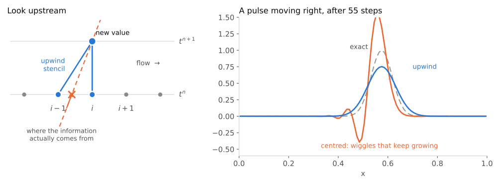
The fix comes from asking where the information actually comes from. If the river flows to the right, the dye at your position a moment from now is the dye that is just upstream of you now. What is downstream can't affect you. So build the derivative from the upstream side only:

$$ \frac{\partial u}{\partial x}\bigg|_i \approx \frac{u_i - u_{i-1}}{h} \quad (a > 0). $$

This is the upwind scheme, published by Courant, Isaacson and Rees in 1952. It is stable as long as the flow moves less than one cell per time step, $|a|\,\Delta t / h \le 1$. That is the CFL condition, named after the paper by Courant, Friedrichs and Lewy from 1928, and it limits the time step of every explicit fluid code ever written.

The price is visible in the figure: upwind smears things out. If you do the Taylor expansion carefully, the upwind scheme is not really solving the advection equation. It is solving

$$ \frac{\partial u}{\partial t} + a\,\frac{\partial u}{\partial x} = \frac{a h}{2}\left(1 - \frac{a\,\Delta t}{h}\right)\frac{\partial^2 u}{\partial x^2}, $$

which is the advection equation plus a diffusion term, the same term as in the heat equation. The scheme is stable because it quietly adds some viscosity, and the amount is set by the grid spacing $h$ rather than by any physics. This numerical diffusion is the main thing everything that follows tries to reduce.

Upwinding when there is no single "upwind"

In a real gas, "which way is the wind blowing" doesn't have a single answer. A disturbance in a moving gas sends out sound waves in both directions, plus a third signal that rides along with the flow and carries differences in density and temperature. Some of the information at a point comes from the left and some from the right.

Sergei Godunov's answer, in 1959, was to stop thinking about derivatives altogether. Store the average of density, momentum and energy in each cell. At each face between two cells there are two different states, one on each side, and the question of what flows through the face becomes a small, self-contained physics problem: two uniform gases, separated by a membrane that is suddenly removed. What happens? This is the Riemann problem, and for the equations of gas dynamics it can be solved exactly.

Left: a space-time diagram of a Riemann problem starting at x = 0.5. A fan of lines spreads to the left (a rarefaction), a dashed line moves slowly to the right (the contact), and a steep line moves faster to the right (the shock). Right: the density at t = 0.2, which falls smoothly through the rarefaction, then has two sharp steps at the contact and the shock. — The Riemann problem that Sod used in 1978 to compare methods, now the standard "shock tube" test. Dense, high-pressure gas on the left and thin gas on the right, with a membrane between them that is removed at $t = 0$. **Left:** three waves spread out from the membrane: a rarefaction (an expansion fan) going left, a contact where the two original gases meet, and a shock going right. **Right:** the density profile these waves create. Godunov's method solves a problem like this one at every cell face, at every time step.

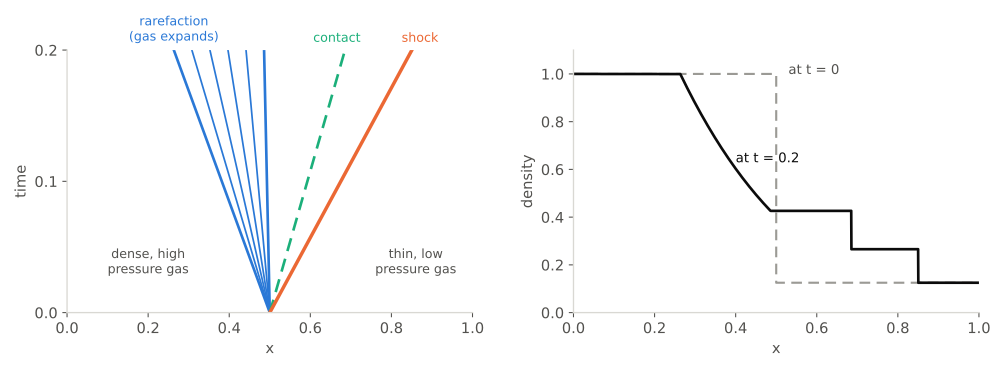
The solution of the Riemann problem tells you which waves cross the face and in which direction, so it does the upwinding for every signal at once. The flux through each face comes from that solution, and the cell averages are updated by what flows in and out. With one value per cell, piecewise constant, Godunov's method reduces to the upwind scheme for the advection equation, and to its proper generalization for gas dynamics.

Solving the exact Riemann problem at every face is expensive, so much of the 1980s went into cheaper approximate solvers that keep the important waves:

Roe (1981) linearizes the problem around an average state.
HLL (Harten, Lax and van Leer, 1983) keeps only the fastest left- and right-going waves and averages everything in between. It is very robust, but it smears contacts.
HLLC (Toro, Spruce and Speares, 1994) puts the contact wave (the "C") back in.
HLLD (Miyoshi and Kusano, 2005) does the same for magnetohydrodynamics, which has more wave families.

For most astrophysical codes, the Riemann solver is the "upwind" half of the method.

Godunov's barrier

Godunov's method is robust, but it is only first order, which means it has all of upwind's smearing. The natural fix, using more neighbours to estimate things more accurately, brings back the wiggles of the centred scheme. Godunov proved in the same 1959 paper that this is unavoidable:

A linear scheme that never creates new maxima or minima can be at most first-order accurate.

"Linear" here means the recipe uses the same fixed weights everywhere. The way around the theorem is to let the scheme look at the data and change its recipe. Use a high-order formula where the solution is smooth, and fall back to something cautious near jumps. Bram van Leer worked this out in a series of five papers between 1973 and 1979, titled Towards the Ultimate Conservative Difference Scheme. Most of the codes in use today are descended from that series.

Reconstruction: getting detail back from averages

The key idea is to split each time step into three parts, sometimes called reconstruct–evolve–average:

Reconstruct. From the cell averages, build a profile inside each cell: a sloped line, a parabola, something more elaborate. Its average over the cell must still equal the stored value.
Evolve. Read off the values that the profiles predict at each face. This gives a left and a right state at every face. Hand them to the Riemann solver and get the fluxes.
Average. Update the cell averages with the fluxes.

Godunov's original method uses the crudest possible reconstruction, a flat value in each cell. Everything that came after it is a smarter answer to step 1.

Six ways to reconstruct a profile from the same cell averages (grey bars). The dotted lines mark the smallest and largest averages. Without a limiter, the straight-line slopes next to the jump overshoot the neighbouring values (orange). After an update, those overshoots become new wiggles. The limited versions choose slopes that never do this. The more aggressive the limiter, the closer the profile gets to the data, but the more it tends to flatten smooth peaks into plateaus.

Piecewise linear and slope limiters

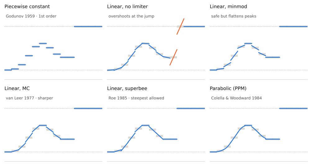
The first step up is a straight line in each cell. Its slope has to come from the neighbours, and there are two obvious candidates: the jump to the left, $\Delta_- = \bar u_i - \bar u_{i-1}$, and the jump to the right, $\Delta_+ = \bar u_{i+1} - \bar u_i$. Averaging them gives a second-order scheme. Near a jump, though, the averaged slope is too steep, and the line reaches above and below the neighbouring values. Those overshoots are exactly the wiggles Godunov's theorem warns about.

A slope limiter is a rule for choosing a safe slope from $\Delta_-$ and $\Delta_+$:

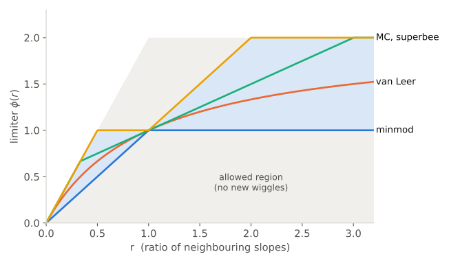
minmod. If the two slopes have the same sign, take the smaller one. If they disagree, so that the cell is a peak or a valley, use zero slope. It is the most cautious choice.
MC ("monotonized central", van Leer 1977). Use the average slope unless it is more than twice either one-sided slope; if it is, cap it there. It is sharper than minmod.
van Leer (1974). The harmonic mean of the two slopes. It is smooth, and it sits between minmod and MC.
superbee (Roe, 1985). The steepest slope that is still allowed. It keeps jumps very sharp, but it also turns smooth hills into mesas.

In 1983 Ami Harten made "never create new wiggles" precise with the notion of a total variation diminishing (TVD) scheme, one whose total up-and-down variation can never grow. In 1984 Peter Sweby drew the picture that is still used to compare limiters.

A plot of limiter function phi against r, the ratio of neighbouring slopes. A grey region shows all choices that avoid new oscillations; a blue band within it shows the choices that are also second-order accurate. Minmod runs along the bottom of the blue band, superbee along the top, and van Leer and MC lie in between. — The Sweby diagram. The horizontal axis is the ratio of the two one-sided slopes, $r = \Delta_-/\Delta_+$, and the vertical axis is how much of $\Delta_+$ the limiter uses as its slope. Any curve inside the grey region creates no new wiggles. The blue band is the part of that region that is also second order. Minmod follows the lower edge of the band and superbee the upper edge. Every limiter is zero for $r < 0$, where the cell is a peak or a valley.

This piecewise-linear family is van Leer's MUSCL scheme (1979), and it is still the default in many codes. The HARM family of general-relativistic MHD codes for black-hole accretion, starting with Gammie, McKinney and Tóth in 2003, uses linear reconstruction with the MC limiter and an HLL-type flux. RAMSES (Teyssier 2002), used for cosmology and galaxy formation, uses a MUSCL-Hancock scheme with a choice of limiters. AREPO (Springel 2010), whose mesh moves with the gas, uses the same piecewise-linear reconstruction and solves Riemann problems on the faces of its moving cells.

Parabolas: PPM

In 1984 Phillip Colella and Paul Woodward published the Piecewise Parabolic Method. Each cell gets a parabola instead of a line. The values at the faces come from a fourth-order interpolation through four neighbouring averages, and then they are adjusted so that the parabola never overshoots the neighbouring data. PPM added a few more pieces aimed at astrophysical flows. It steepens contact discontinuities, which don't sharpen themselves the way shocks do, so the edge between two different gases stays sharp. It flattens the profile right at strong shocks, which stops the small post-shock oscillations that higher-order schemes tend to produce.

PPM became the standard in astrophysics. A short history:

PROMETHEUS (Fryxell, Müller and Arnett, 1989) brought PPM to supernova modelling. Its first big result was showing how the layers of SN 1987A mix through Rayleigh–Taylor instabilities.
VH-1 (Blondin and collaborators) is also PPM-based. It is the hydro solver inside the CHIMERA core-collapse supernova code.
FLASH (Fryxell et al. 2000) took over the PROMETHEUS hydro and became a workhorse for thermonuclear (Type Ia) supernovae and astrophysical combustion.
Enzo, used for cosmology and star formation, CASTRO, used for stellar explosions, and Athena and Athena++, used for MHD and accretion, all offer PPM, and it is often their default.

Beyond parabolas: ENO, WENO and friends

What about even higher order? Using a wider stencil for a cubic or a quartic runs into trouble when the stencil straddles a jump. The ENO ("essentially non-oscillatory") idea of Harten, Engquist, Osher and Chakravarthy (1987) is to try several candidate stencils and use the smoothest one, so that the interpolation never reaches across a discontinuity.

WENO ("weighted ENO": Liu, Osher and Chan 1994; Jiang and Shu 1996) takes a weighted blend of all the candidates instead. In smooth regions the weights combine three third-order stencils into one fifth-order formula (WENO5). Near a jump, the weight on any stencil that crosses it drops almost to zero. WENO5 is not strictly TVD: it can produce tiny over- and undershoots, which is what "essentially" means. In exchange, it keeps smooth features far better than any limiter. Other schemes in the same spirit include MP5 (Suresh and Huynh, 1997), which is used in some numerical-relativity codes for neutron-star mergers, such as WhiskyTHC. PLUTO (Mignone et al. 2007) offers several of these alongside PPM.

Putting them side by side

The classic way to compare reconstructions is the test from Jiang and Shu's 1996 paper. It is a row of shapes that are each hard in a different way: a narrow smooth peak, a square pulse, a triangle with a sharp tip, and a half-ellipse with infinite slope at its edges. Move them around a periodic domain and compare the result with where they started.

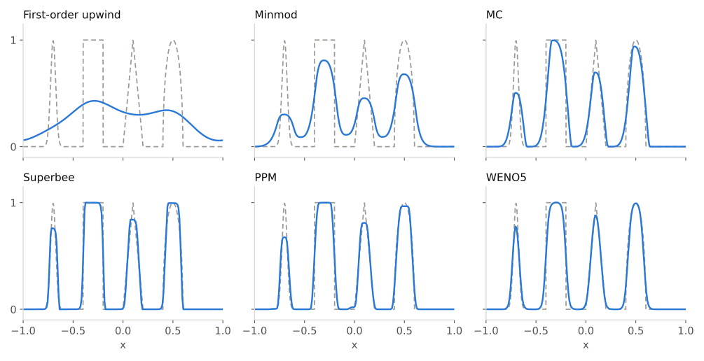
The Jiang–Shu test: four shapes carried twice around a periodic domain on 200 cells. Every scheme uses the same upwind flux and the same three-stage Runge–Kutta time stepping; only the reconstruction changes. First-order upwind has diffused everything into a blur. Minmod clips the peaks. Superbee keeps the square pulse almost perfect, but it squares off the smooth peak and the triangle. PPM and WENO5 do best overall, and WENO5 keeps the narrow peak highest.

The figure shows the trade-off that every choice in this area makes. A scheme that is aggressive enough to keep jumps sharp tends to damage smooth features, and a scheme that is gentle on smooth features smears jumps.

The limiters have one more weakness. They all set the slope to zero at peaks and valleys, because they can't tell a genuine smooth maximum from the start of an oscillation. So even on perfectly smooth data, a slope-limited scheme loses accuracy at every extremum. You can measure this by moving a sine wave once around the domain and watching how the error shrinks as the grid is refined.

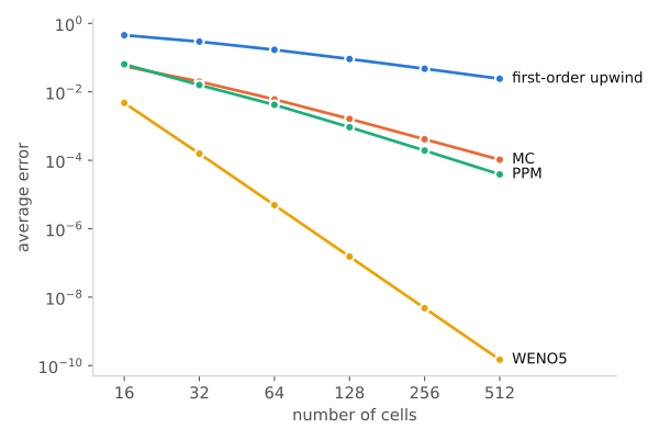
Log-log plot of average error against number of cells, from 16 to 512. First-order upwind falls slowly. MC and PPM fall faster and nearly together. WENO5 falls much faster, reaching about 1e-10 at 512 cells. — Error after moving a sine wave once around the domain. Each doubling of the grid cuts the error by about 2 for first-order upwind (first order), by about 4 to 5 for MC and PPM (roughly second order: their limiters clip the crests of the wave), and by 32 for WENO5 (fifth order). At 512 cells WENO5 is nearly a million times more accurate than MC. The time step was shrunk on the finer grids so that the time stepping didn't hide the difference.

Clipping at extrema is why "extremum-preserving" versions of PPM appeared later (Colella and Sekora, 2008), and why groups that care about smooth waves, such as those computing gravitational waves from merging neutron stars, often prefer WENO or MP5.

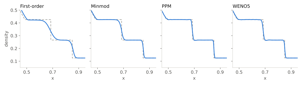
Back to gas dynamics. Here is Sod's shock tube from earlier, run with four of the reconstructions:

Four panels zoomed on the contact and shock in the Sod shock tube. First order smears the contact over many cells and the shock over fewer. Minmod is sharper. PPM and WENO5 capture both in two or three cells. — Density in Sod's shock tube at $t = 0.2$, on 200 cells with the HLLC Riemann solver, zoomed in on the contact (left step) and the shock (right step). The first-order scheme smears the contact much more than the shock. A shock squeezes itself sharp, while a contact just drifts and diffuses. Higher-order reconstruction fixes most of this.

What doesn't show up in the plots

A few practical details matter as much as the choice of scheme:

What you reconstruct. You can reconstruct the conserved variables (density, momentum, energy), the primitive ones (density, velocity, pressure), or the characteristic variables (the amplitudes of each wave family). Primitive variables are the usual choice, because they make it easy to keep pressure and density positive. Characteristic variables give the cleanest results near shocks, at extra cost.
Positivity. In astrophysics, a near-vacuum is often right next to something extremely dense: the surface of a star, the atmosphere around a neutron star, the funnel above a black hole. A reconstruction that undershoots by a tiny amount there can produce a negative density or pressure, and the code crashes. Production codes carry "floors" and fallbacks that drop to first order in trouble spots.
Not everyone upwinds. The old alternative is to use centred differences and add an explicit artificial viscosity to damp the wiggles. The idea goes back to von Neumann and Richtmyer at Los Alamos in 1950. The ZEUS code (Stone and Norman, 1992), which ran a large share of astrophysical MHD in the 1990s, uses that approach, together with van Leer–style upwind interpolation for moving material between cells. Smoothed particle hydrodynamics (SPH) also traditionally relies on artificial viscosity. Even so, newer particle methods such as GIZMO (Hopkins, 2015) solve Riemann problems between neighbouring particles. The Godunov idea has spread well beyond grids.

In short

Upwinding is the physics: information travels along definite directions, and a stable scheme has to respect them. For a single equation that means looking upstream. For a gas it means solving a Riemann problem at every face. Reconstruction is the accuracy: getting more out of cell averages without creating oscillations. Godunov's theorem says you can't have both for free with a fixed recipe, so every modern scheme adapts to the data.

Shock-capturing codes have been tuned in this way for some seventy years, and when you see "PPM + HLLC" or "WENO5 + HLLD" in a paper, you now know what that line means.