Finite differences, finite volumes and finite elements

In 1916, while driving an ambulance on the Western Front, Lewis Fry Richardson tried to forecast the weather by hand. He took the measured state of the atmosphere over central Europe at 7 a.m. on 20 May 1910, wrote down the equations of fluid flow, and replaced every derivative with a difference between numbers at neighbouring points on a grid. Working with pencil and paper in a rest billet, it took him about six weeks to forecast six hours ahead. His answer was a pressure rise of 145 hPa, about a seventh of the weight of the entire atmosphere, when in reality the pressure barely moved.

The forecast was wrong (mostly because of noise in the starting data, it later turned out), but the method was right. Today a supercomputer does Richardson's arithmetic billions of times a second, and nearly every simulation you have heard of, from weather to aircraft to crash tests to exploding stars, starts with the same problem he faced:

Physics is written as differential equations about smooth, continuous quantities. A computer can only do arithmetic on a finite list of numbers.

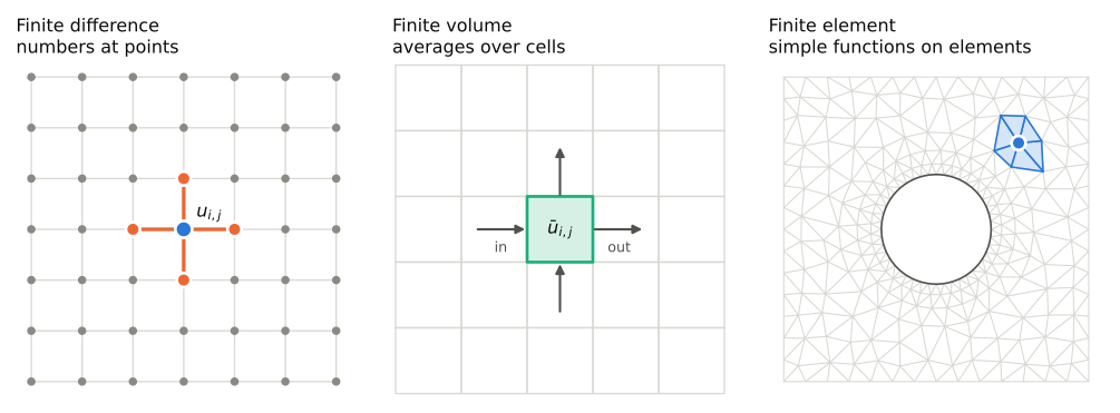
Turning one into the other is called discretization, and there are three big families of methods for doing it: finite differences, finite volumes and finite elements. They differ in one basic choice: what does each number in the computer's list actually mean?

Three panels: a regular grid of points with a five-point stencil; a grid of square cells with arrows showing flux in and out of one cell; an irregular triangular mesh around a circular hole with one node's triangles highlighted. — The three ways of storing a continuous field in a computer. **Left:** finite difference stores values at grid points and combines each point with its neighbours (orange). **Middle:** finite volume stores the average over each cell and tracks what flows across its faces. **Right:** finite element breaks the domain into elements of any shape (here, a plate with a hole) and builds the solution from simple functions; the highlighted triangles are where one node's function is non-zero.

A running example: heat in a rod

To keep things concrete, take a metal rod with some temperature profile $u(x, t)$ along it. Heat flows from hot to cold, and the equation that describes it is the heat equation:

$$ \frac{\partial u}{\partial t} = \kappa \frac{\partial^2 u}{\partial x^2} $$

In words: the temperature at a point changes at a rate set by its curvature. If a point is hotter than the average of its surroundings (a peak, where $\partial^2 u/\partial x^2 < 0$), it cools down. If it's colder (a dip), it warms up. The constant $\kappa$ says how quickly heat diffuses through the material.

The difficulty is that $u$ has a value at every one of the infinitely many points along the rod. Each method below replaces that with finitely many numbers.

Finite differences: numbers at points

This is Richardson's method, and the most direct one. Put points along the rod, spaced a distance $h$ apart, and store the temperature at each: $u_0, u_1, u_2, \ldots$ Then replace every derivative with a difference between neighbouring values.

The slope at a point is approximately "rise over run" between nearby points. The simplest choice uses the next point over (a forward difference),

$$ \frac{\partial u}{\partial x}\bigg|_i \approx \frac{u_{i+1} - u_i}{h}, $$

but you do much better by looking symmetrically to both sides (a central difference):

$$ \frac{\partial u}{\partial x}\bigg|_i \approx \frac{u_{i+1} - u_{i-1}}{2h}. $$

Left: a curve with its true tangent at x, a forward-difference line through x and x+h, and a central-difference line through x-h and x+h that is nearly parallel to the tangent. Right: log-log plot of slope error against h; the forward-difference error falls proportionally to h and the central-difference error proportionally to h squared. — **Left:** estimating the slope at $x$ from neighbouring points. The central difference (orange) is almost parallel to the true tangent; the forward difference (blue) is visibly off. **Right:** what happens as the spacing $h$ shrinks. Halving $h$ halves the forward-difference error but cuts the central-difference error by a factor of four, because its error is proportional to $h^2$. This "order of accuracy" is the main way numerical methods are compared.

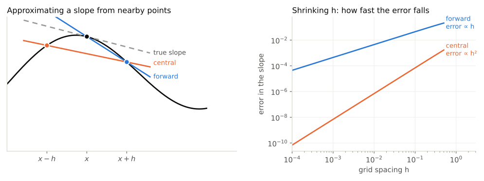
Apply the same idea twice and you get the second derivative, which only needs a point and its two neighbours:

$$ \frac{\partial^2 u}{\partial x^2}\bigg|_i \approx \frac{u_{i+1} - 2u_i + u_{i-1}}{h^2}. $$

Notice that this is just "the average of the neighbours minus the point itself", scaled by $1/h^2$, which is exactly the "am I hotter than my surroundings?" test in the heat equation. Do the same for time, with a small time step $\Delta t$, and the heat equation becomes an update rule a child could follow:

$$ u_i^{\text{new}} = u_i + \frac{\kappa\,\Delta t}{h^2}\left(u_{i+1} - 2u_i + u_{i-1}\right). $$

Every point looks at its neighbours, nudges itself towards their average, and repeats. In two or three dimensions the same pattern gives the five-point (or seven-point) "stencil" in the left panel of the first figure.

Strengths. Finite differences are simple to understand, simple to code and very fast. On a regular grid it is easy to reach high accuracy by using wider stencils.

Weaknesses. The method assumes a tidy, regular grid. Curved boundaries like the air around a wing or a hole in a plate are awkward: the boundary falls between grid points. And because it only thinks about point values, it doesn't automatically conserve quantities like mass or energy, and it struggles badly with sudden jumps, as we'll see shortly.

Where it's used.

Electromagnetics. The finite-difference time-domain method (Kane Yee, 1966) is a workhorse for designing antennas, phone and radar hardware, and for studying how light moves through nanostructures.
Seismic imaging. Oil and gas exploration and earthquake hazard studies simulate sound waves bouncing through layers of rock, typically on big regular grids where finite differences are fast.
Weather. Some widely used research weather models, such as WRF, are built on finite differences on regular (staggered) grids.
Black holes. Many of the numerical-relativity codes that simulated merging black holes, producing the waveforms LIGO used to recognise real signals, are high-order finite-difference codes.
Finance. The Black–Scholes equation for option prices is a heat equation in disguise, and is routinely solved with finite differences.

Finite volumes: averages over cells

Finite volume starts from a different observation. Most laws of physics are really conservation laws: mass, momentum and energy aren't created or destroyed, only moved around. So instead of storing the value at a point, cut space into little cells and store the average over each cell, $\bar u_i$. Then apply the conservation law to each cell as bookkeeping:

$$ \frac{d \bar u_i}{dt} = \frac{F_{i-1/2} - F_{i+1/2}}{h}, $$

or in words: the amount in a cell changes only by what flows in through one face minus what flows out through the other. Here $F_{i \pm 1/2}$ is the flux, the rate at which heat (or mass, or momentum) crosses each face between cells.

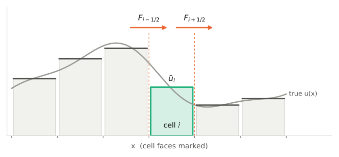
A smooth curve u(x) with the domain cut into six cells, each drawn as a bar whose height is the cell average. Cell i is highlighted, with flux arrows labelled F i-1/2 and F i+1/2 at its left and right faces. — Finite volume replaces the smooth profile (grey) with one average per cell (bars). The average in cell $i$ changes only through the fluxes $F_{i-1/2}$ and $F_{i+1/2}$ at its two faces.

The key point is that the flux leaving cell $i$ through its right face is the exact same number as the flux entering cell $i+1$ through its left face. Add up all the cells and every internal flux cancels in pairs. Whatever the rest of the approximation gets wrong, nothing leaks: the total is conserved to the last decimal place, which a finite-difference scheme does not guarantee.

The real payoff comes with shocks: sudden jumps, like the shock wave in front of a supersonic jet or the edge of an exploding star. A derivative at a jump is infinite, so anything built on Taylor expansions at points gets confused. Averages and fluxes, though, still make perfect sense across a jump. Starting with Sergei Godunov in 1959, people learned to compute the flux at each face by solving a tiny "what happens when two different states collide?" problem, and to add limiters that stop the scheme from creating new wiggles near steep jumps.

Three panels showing a square pulse and a smooth bump carried once around a periodic domain. A simple first-order scheme smears both shapes out. A simple second-order scheme keeps the bump but produces oscillations and overshoots around the square pulse. A finite-volume scheme with a limiter keeps the square pulse sharp with no overshoot and keeps the bump. — The same test for three schemes: carry a square pulse and a smooth bump once around a loop, so the exact answer (dashed) is just the starting shape. A simple first-order scheme (**left**) smears everything. A simple second-order scheme (**middle**) keeps the smooth bump but rings around the jumps and overshoots, which in a real simulation could mean negative density. The finite-volume scheme with a limiter (**right**) keeps the jumps sharp with no overshoot. All three ran on the same 200 cells.

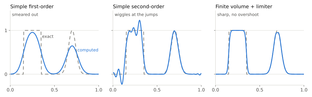
Strengths. Exact conservation, robust handling of shocks, and it works on unstructured meshes of any cell shape. For anything that flows, this combination is hard to beat.

Weaknesses. It is harder to push to very high accuracy than finite differences on smooth problems, and the mathematics guaranteeing it converges is less tidy than for finite elements.

Where it's used.

Engineering fluid dynamics. The big commercial and open-source CFD packages (ANSYS Fluent, OpenFOAM, STAR-CCM+) are finite-volume codes. They design aircraft, car bodies, Formula 1 aerodynamics, turbines, ventilation systems and blood pumps.
Weather and climate. The US National Weather Service's Global Forecast System has run on FV3, a Finite-Volume Cubed-Sphere core, since 2019, and many climate models' atmosphere and ocean components are finite volume.
Astrophysics. Simulations of supernovae, star formation, accretion disks and colliding galaxies are full of shocks, so most astrophysical (magneto)hydrodynamics codes are shock-capturing finite-volume codes.

Finite elements: simple functions stitched together

Finite element takes yet another view. Instead of approximating the equation at points or cells, it approximates the solution itself as a sum of simple building blocks.

Cut the domain into elements (intervals in 1D, triangles or tetrahedra in 2D and 3D) of whatever size and shape you like. At each node put a "hat" function $\varphi_i(x)$ that equals 1 at that node, falls linearly to 0 at the neighbouring nodes, and is zero everywhere else. Any approximate solution is then a weighted sum of hats:

$$ u_h(x) = \sum_i u_i \, \varphi_i(x), $$

which is just a connect-the-dots curve through the values $u_i$ at the nodes.

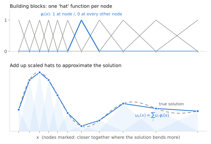
Top: a row of triangular hat functions on unevenly spaced nodes, closer together on the left; one is highlighted. Bottom: the true solution as a dashed curve and its piecewise-linear finite-element approximation through the nodes, built by adding scaled hats. — **Top:** one hat function per node; note the nodes don't need to be evenly spaced. **Bottom:** scaling each hat by the value at its node and adding them up gives a piecewise-linear approximation (blue) of the true solution (dashed). Putting nodes closer together where the solution bends sharply spends the effort where it's needed.

How do we find the weights $u_i$? A connect-the-dots function has kinks, so its second derivative isn't even defined at the nodes, and we can't ask it to satisfy the equation at every point. Instead we ask for something weaker: that the equation hold on average, when weighted by each hat function in turn. Multiplying by $\varphi_i$, integrating, and doing one integration by parts moves one derivative onto the hat, so only first derivatives are ever needed. This is called the weak form, and it produces one equation per node, a big linear system of the form $K\mathbf{u} = \mathbf{f}$. (For structures, $K$ is literally called the stiffness matrix, a leftover from the method's origins.)

Strengths. Elements can be any shape and size, so finite elements fit complicated geometry naturally (the plate with a hole in the first figure, an engine block, a hip bone) and can use small elements only where the solution changes quickly. The method also rests on solid mathematics: you can prove how large the error is and estimate it during a run, which matters when a bridge depends on the answer.

Weaknesses. It's more complicated to implement, and it means solving large coupled systems of equations rather than updating each point from its neighbours. The classic version also isn't designed for shocks, which is why fluid dynamics leaned towards finite volumes.

Where it's used.

Structural engineering. This is where the method grew up: aerospace engineers at Boeing in the 1950s analysed wing panels this way, and Ray Clough coined the name "finite element" in 1960 (Richard Courant had sketched the idea back in 1943). Today it checks bridges, skyscrapers, aircraft frames and wind-turbine blades.
Crash testing. Codes like LS-DYNA crash virtual cars thousands of times before a real one hits a wall.
Medicine. Stresses in hip implants, dental crowns and bone, blood flow in patient-specific arteries, and electric fields in the brain for neurostimulation.
Electronics and multiphysics. Heat flow in chips, electromagnetic fields in motors and MRI coils, and coupled problems in packages like COMSOL and ANSYS Mechanical.

The surprise: sometimes they're the same

Go back to the simplest problem, the steady temperature in a rod with a heat source $f$, i.e. $-u'' = f$, on evenly spaced points:

Finite difference replaces $u''$ directly:

$$ -\frac{u_{i+1} - 2u_i + u_{i-1}}{h^2} = f_i. $$

Finite volume integrates over cell $i$ and approximates the flux $u'$ at each face by $(u_{i+1}-u_i)/h$:

$$ -\frac{1}{h}\left[\frac{u_{i+1}-u_i}{h} - \frac{u_i-u_{i-1}}{h}\right] = f_i, $$

which is the same thing.

Finite element with hat functions gives a stiffness matrix whose rows are $\tfrac{1}{h}\,(\ldots,\,{-1},\ 2,\ {-1},\,\ldots)$, and a right-hand side close to $h f_i$. Divide by $h$:

$$ \frac{-u_{i-1} + 2u_i - u_{i+1}}{h^2} = f_i. $$

The same equations again.

Three different philosophies, one set of equations. So the differences aren't in the arithmetic of easy problems. They're in what each method assumes the solution looks like between the numbers, and that matters on hard problems: curved boundaries, jumps, quantities that must be conserved, and solutions that need fine detail in some places but not others.

Side by side

	Finite difference	Finite volume	Finite element
Each number means	value at a point	average over a cell	weight of a basis function
Natural mesh	regular grid	any cells	any elements (triangles, tetrahedra, …)
Conserves exactly	not automatically	yes, by construction	not automatically (standard form)
Shocks and jumps	poor	excellent	needs special variants
Complex geometry	awkward	good	excellent
Ease of coding	easiest	moderate	hardest
Typical home	waves, simple domains, high accuracy	fluids, gases, plasmas, astrophysics	solids, structures, heat, electromagnetics

A rough rule of thumb:

If it flows and might form shocks (air, water, gas, plasma), reach for finite volume.
If it has a complicated shape and a fairly smooth solution (a loaded beam, a heated engine part, a field around a device), reach for finite element.
If the domain is a simple box and you want speed and high accuracy (waves, smooth fields), finite difference is hard to beat.

The lines blur in practice. Discontinuous Galerkin methods, for example, use finite-element-style functions inside each cell and finite-volume-style fluxes between cells, getting much of both. But nearly every simulation code you'll come across is built on one of these three ideas, and once you know what its numbers mean, you know a lot about what it's good at and where it will struggle. Richardson would be pleased that his six weeks of arithmetic now takes a few seconds.