Boltzmann transport in astrophysical simulations: light first, then neutrinos

The last few posts were about gas: how to move it, how to put a grid under it. But a lot of what happens in astrophysics is not done by the gas. It is done by particles that fly through the gas at the speed of light and barely notice it most of the time: photons, and in the densest places, neutrinos. Light carries the energy out of a star and sets its structure. Radiation pressure limits how fast a black hole can grow. And in a core-collapse supernova the neutrinos carry away 99% of the energy, and the few percent they leave behind in the gas is what blows the star up. If you want to simulate any of this, you have to simulate the transport.

This post is about what that problem looks like, before any approximations. I'll build it up with light, because everyone has an intuition for light, and then go through what changes for neutrinos. The next post is about why the neutrino version is so hard, and the one after that is about the tricks people use to get around it.

Why radiation is not a fluid

The reason gas is easy is collisions. In a cell of gas the particles bounce off each other constantly: in air, each molecule collides about ten billion times a second. That keeps the velocities in a Maxwell distribution, and a Maxwell distribution is fixed by three numbers: density, mean velocity and temperature. So a cell of gas is five numbers (density, three velocity components, energy), and the equations of hydrodynamics tell you how those five numbers change. Everything about the individual particles has been averaged out, and nothing was lost.

Photons don't collide with each other at all, and they interact with the gas only when they happen to hit something. How far a photon flies between interactions, the mean free path, is not a universal number: it is centimetres in the centre of the Sun, light years in a molecular cloud, and effectively infinite in intergalactic space. Where the mean free path is short, radiation behaves like a fluid in equilibrium with the gas and you can describe it with a temperature. Where it is long, the photons at a point remember where they came from. A point in the solar wind receives sunlight from one direction and nothing from the others, and no temperature describes that. You have to keep track of which direction the radiation is going and what energy it has, separately, at every point.

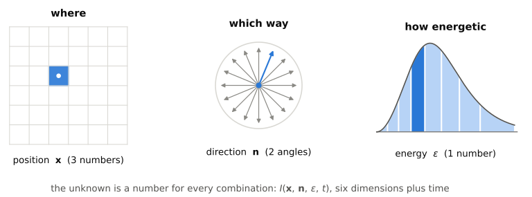
Three panels: a spatial grid with one cell highlighted; a circle of arrows showing the possible directions at that point; and a spectrum divided into energy bins. Together they show the six coordinates of the specific intensity. — The unknown in a transport problem. Gas needs five numbers per cell. Radiation needs a number per cell *and* per direction *and* per energy: a function on a six-dimensional space, evolving in time.

So the thing we solve for is not a few numbers per cell but a whole function: the distribution function $f(\mathbf{x}, \mathbf{p}, t)$, the number of particles per unit volume of position space per unit volume of momentum space. Three coordinates for where, three for the momentum (which for a massless particle means two angles for the direction $\mathbf{n}$ and one number for the energy $\varepsilon = h\nu$). Six dimensions plus time. Astronomers usually work with an equivalent quantity, the specific intensity $I_\nu(\mathbf{x}, \mathbf{n}, t)$: the energy flowing per unit time, per unit area perpendicular to $\mathbf{n}$, per unit solid angle around $\mathbf{n}$, per unit frequency. The two are proportional, $I_\nu = (2h\nu^3/c^2)\, f$ for photons, so pick whichever makes the formulas shorter.

The transfer equation

Imagine a thin pencil of radiation travelling through some material in the direction $\mathbf{n}$, and ask how the intensity along it changes. Four things can happen to it.

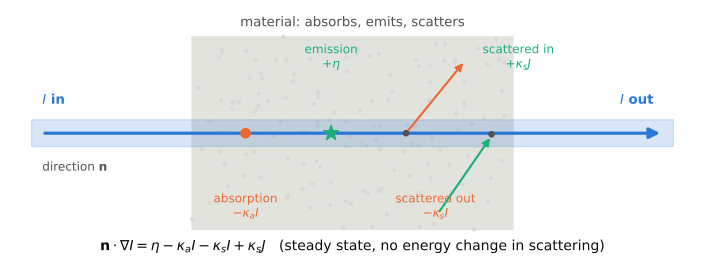
A beam of radiation crossing a slab of material. Along the beam, a photon is absorbed, a new one is emitted into the beam, one is scattered out of the beam, and one from elsewhere is scattered into it. — The four terms of the transfer equation. Absorption and out-scattering remove energy from the beam in proportion to how much is there; emission and in-scattering add energy, and don't care what the beam was doing. $J$ is the intensity averaged over all directions.

The material can absorb photons out of the beam. It does so at a rate proportional to the intensity (twice the photons, twice the absorptions), so this is a loss $-\kappa_a I$, where $\kappa_a$ is the absorption coefficient, an inverse length. It can emit photons into the beam, a gain $+\eta$ that depends on the material's temperature and composition but not on $I$. It can scatter photons out of the beam into other directions, another loss proportional to $I$, say $-\kappa_s I$. And it can scatter photons that were going other ways into the beam, a gain that depends on how much radiation is arriving from everywhere else; for scattering that sends photons equally in all directions, that is $+\kappa_s J$ with $J$ the average of $I$ over directions.

Put these together and let the beam evolve in time, and you get the equation of radiative transfer:

$$ \frac{1}{c}\frac{\partial I}{\partial t} + \mathbf{n}\cdot\nabla I = \eta - (\kappa_a + \kappa_s)\, I + \kappa_s J . $$

The left side says that, left alone, the intensity is simply carried along straight lines at the speed of light. The right side is everything the material does to it. Written in terms of $f$ this is

$$ \frac{\partial f}{\partial t} + c\,\mathbf{n}\cdot\nabla f = \mathcal{C}[f], $$

which is the Boltzmann equation: free streaming on the left, a collision term on the right. It is the same equation that describes a dilute gas, just with the particle speed fixed to $c$ and with the collisions being between the photons and the gas rather than among the photons themselves. If the particles have mass, or there is gravity bending their paths, the left side gains a term for the change of momentum along the path, $\dot{\mathbf{p}}\cdot\partial f/\partial\mathbf{p}$. In general relativity the straight lines become geodesics and the energy shifts as the particle climbs out of the potential well. The structure stays the same.

Notice what the equation is not. It is linear in $I$ if the material is given: twice the radiation, twice the absorption. It has no pressure term, no sound waves, no shocks. Compared to hydrodynamics it is almost trivially simple in form. All the difficulty is in the number of dimensions and in the range of the coefficients.

Optical depth

The absorption coefficient has units of inverse length, so its inverse is a length: the mean free path, $\lambda = 1/\kappa$. The natural way to measure distance along a beam is in mean free paths. That dimensionless distance is the optical depth,

$$ \tau = \int \kappa \, \mathrm{d}s . $$

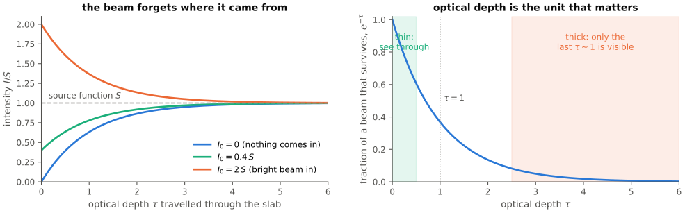
If the material only absorbs and emits, with the emission written as $\eta = \kappa_a S$ where $S$ is called the source function (for matter in thermal equilibrium $S$ is the Planck function at the local temperature), the steady transfer equation along the beam is $\mathrm{d}I/\mathrm{d}\tau = S - I$, and you can solve it:

$$ I(\tau) = I_0\, e^{-\tau} + \int_0^{\tau} S(\tau')\, e^{-(\tau-\tau')}\,\mathrm{d}\tau' . $$

Whatever came in is attenuated by $e^{-\tau}$, and the material along the way adds its own emission, with the parts further back attenuated more.

Left: the intensity along a beam through a uniform slab, for three different incoming intensities; all converge on the source function within a few optical depths. Right: the surviving fraction of a beam, exp(-tau), with the thin and thick regimes marked. — Left: for a uniform slab with source function $S$, whatever enters relaxes to $S$ within two or three optical depths. Right: a beam is attenuated by $e^{-\tau}$, so when you look into an opaque object you see roughly its last optical depth. The Sun's photosphere is the layer where $\tau$ reaches about one.

Two limits fall out immediately.

Optically thin, $\tau \ll 1$. Almost nothing happens to the radiation; it streams freely. The intensity at a point is whatever the sources in view are emitting, and there can be radiation going in one direction and none in the others. The solar wind, a supernova remnant, the gas between galaxies.

Optically thick, $\tau \gg 1$. The radiation has been absorbed and re-emitted so many times that it has forgotten everything except the local temperature. It is nearly isotropic, with a slight excess in the direction in which the temperature falls, and that excess is what carries energy. In this limit the transfer equation collapses to a diffusion equation: the flux is proportional to the gradient of the energy density,

$$ \mathbf{F} = -\frac{c}{3\kappa}\nabla E , $$

with a diffusion coefficient $c\lambda/3$. The interior of a star, where a photon random-walks for tens of thousands of years to cover a distance it could fly in two seconds.

Both limits are easy to compute. The optically thin limit is ray tracing; the thick limit is a heat equation. The trouble is that every interesting astrophysical object contains both, and the physics usually happens in the layer between them, where $\tau$ is around one and neither picture works. A stellar photosphere, the surface of an accretion disk, the edge of an ionized bubble, and, as we'll see, the layer of a supernova where the neutrinos deposit their energy.

Moments and the closure problem

You rarely want the full angular distribution; you want its consequences for the gas. The gas feels the radiation through a few averages over direction, the moments of $I$:

$$ E = \frac{1}{c}\int I\,\mathrm{d}\Omega, \qquad \mathbf{F} = \int I\,\mathbf{n}\,\mathrm{d}\Omega, \qquad \mathsf{P} = \frac{1}{c}\int I\,\mathbf{n}\mathbf{n}\,\mathrm{d}\Omega . $$

$E$ is the radiation energy density, $\mathbf{F}$ the flux (energy per area per time), and $\mathsf{P}$ the radiation pressure tensor. The gas gains energy at a rate set by $E$ and loses it by emission, and it feels a force from the flux: $(\kappa/c)\mathbf{F}$ per unit volume is the radiation force that holds up the most luminous stars and drives their winds.

Integrate the transfer equation over all directions and you get an equation for $E$ whose flux is $\mathbf{F}$. Multiply by $\mathbf{n}$ first and integrate, and you get an equation for $\mathbf{F}$ whose flux is $\mathsf{P}$:

$$ \frac{\partial E}{\partial t} + \nabla\cdot\mathbf{F} = 4\pi\eta - c\kappa_a E, \qquad \frac{1}{c^2}\frac{\partial \mathbf{F}}{\partial t} + \nabla\cdot\mathsf{P} = -\frac{\kappa}{c}\mathbf{F} . $$

These look like fluid equations: a conservation law for energy, one for momentum. But each equation involves the next moment up, and the series never closes on its own. To use them you need a rule for $\mathsf{P}$ in terms of $E$ and $\mathbf{F}$, a closure. The ratio $P/E$ along the direction of the flux is called the Eddington factor, and the whole difficulty of moment methods is guessing it.

The two limits again tell you what it should be. Deep inside, where the radiation is isotropic, the pressure is the same in all directions and $P = E/3$ (just like a gas of particles moving at speed $c$). Far outside, where all the radiation streams one way, $P = E$ along that direction and nothing across it. In between it moves from one to the other, and how it does so depends on the geometry of the sources.

There is one case where you can see the whole transition exactly: a uniform sphere that emits and absorbs with a constant $\kappa$, and nothing outside. For every radius and direction the intensity is just $B\,(1 - e^{-\kappa s})$ where $s$ is the length of the path through the sphere that ends at that point in that direction, which is a few lines of geometry. The figure below shows what the radiation field looks like, and how the moments behave, for a sphere four mean free paths in radius.

Left: the intensity as a function of direction cosine at five radii in and around a uniform emitting sphere; it is flat at the centre and becomes a narrow cone of outgoing directions far outside. Right: the Eddington factor rises from 1/3 inside the sphere to 1 far away, and the flux factor rises from 0 to 1. — The radiation field of a uniform sphere with $\kappa R = 4$. At the centre the intensity is the same in all directions. Near the surface, looking outward ($\mu > 0$) you see the full emission, looking inward you see less because the path through the sphere is shorter. Outside, radiation arrives only from the cone that the sphere subtends, and the cone narrows with distance. The moments on the right track this: diffusion inside, free streaming far away, and a transition that takes several radii to complete. Astrophysical transport lives in that transition.

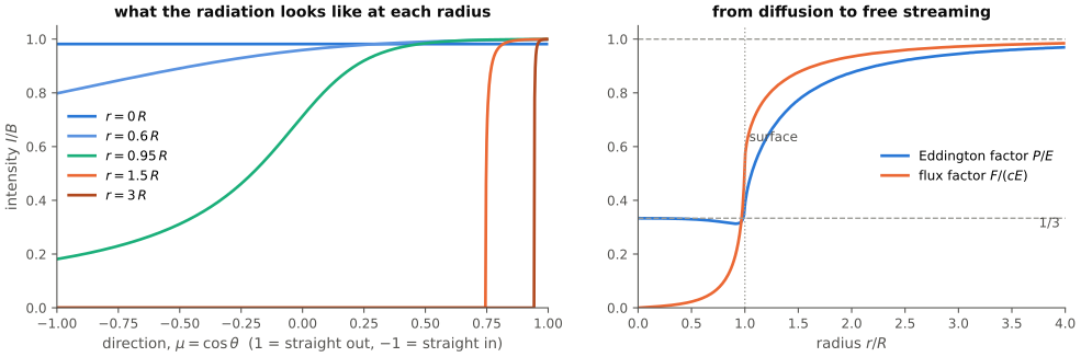
Hold onto this picture. It is the test problem every closure is judged against, and it comes back in the third post.

Where this shows up

The transfer equation was written down for stellar atmospheres: the spectrum you see from a star is produced in the layer where $\tau$ passes through one, and predicting it (and therefore reading a star's temperature, gravity and composition off its spectrum) means solving transport through that layer, one frequency at a time, with thousands of spectral lines. That is still the bulk of what "radiative transfer" means to most astronomers, and it is a problem in a static, one-dimensional atmosphere.

In simulations the radiation is coupled to moving gas, and then it does things. In star formation, the light of a newly formed massive star heats and ionizes the cloud it formed in and its pressure pushes the gas away, which decides how big the star can get and when the cloud stops forming stars. In accretion disks around black holes, radiation carries away the energy released by infall and also, when the disk is bright enough, holds the disk up against gravity. In cosmology, ultraviolet light from the first galaxies ionized the hydrogen of the whole universe, and simulating that means transporting photons across a box hundreds of millions of light years on a side. In supernovae and in the kilonovae that follow neutron star mergers, the light curve we observe is the result of photons diffusing out through expanding, radioactive ejecta, and the code that produces the light curve is a transport code.

Each of these has its own balance of thin and thick, and its own simplifications that happen to be good enough. Which brings us to the one that has the fewest.

Neutrinos: the same equation in a worse place

A neutrino is a particle with a direction and an energy that flies through matter until it hits something. The Boltzmann equation above describes it exactly, with the collision term replaced by the weak-interaction rates. In most of the universe neutrinos simply leave; the Sun is transparent to them, which is why they are useful for seeing its core. There are three places where the matter is dense enough to stop them: the core of a massive star in the half-second after it collapses, the remnant of two neutron stars merging, and the disk that forms when a collapsing massive star has enough spin to make one, a collapsar. In all three, the neutrinos are not a side effect. They carry away most of the energy, they decide how much of the matter is protons versus neutrons (and therefore what elements get made), and in the supernova case they are what revives the stalled shock.

Here is what changes from the photon problem.

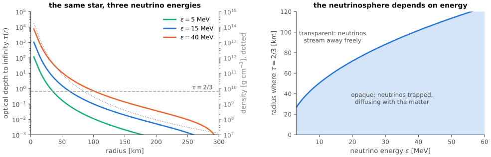
The cross sections depend strongly on energy. The weak interaction cross sections grow as the square of the neutrino energy: $\sigma \sim 10^{-44}\,\mathrm{cm^2}\,(\varepsilon / m_e c^2)^2$. A 40 MeV neutrino is sixty times more likely to interact than a 5 MeV one. So there is no single "surface" of the proto-neutron star where neutrinos decouple. There is a different neutrinosphere for every energy, and the high-energy neutrinos decouple further out, where it is cooler, than the low-energy ones. You cannot average over energy without losing the physics, and the energy dimension of the phase space has to be kept.

A toy proto-neutron star: density falling from $3\times10^{14}\,\mathrm{g\,cm^{-3}}$ at the centre, and an opacity proportional to density and to energy squared. The radius where the optical depth to infinity drops below 2/3, which is roughly where neutrinos of that energy escape, moves from about 35 km for 5 MeV to about 100 km for 40 MeV. The numbers are illustrative; the trend is real.

The particles are fermions. A neutrino cannot be scattered into a state that is already occupied, so every rate carries a blocking factor $(1 - f)$ for the final state. The collision term becomes nonlinear in $f$. Deep inside the proto-neutron star the neutrinos are degenerate, with $f$ close to one, and blocking changes the rates by large factors.

There are several species, and they talk to each other. Electron neutrinos, electron antineutrinos, and the four heavy-lepton species (usually lumped together as $\nu_x$) have different interactions. The $\nu_e$ and $\bar\nu_e$ are absorbed on neutrons and protons, which changes the proton fraction of the matter; the $\nu_x$ only scatter. Pairs of all kinds are created from electron-positron annihilation and from nucleon-nucleon bremsstrahlung, and the reverse processes couple the species. On top of that, electron-lepton number is conserved, so the transport has to track a number flux as well as an energy flux, and track it exactly: a leak of lepton number is a leak of the quantity that sets the composition.

The hard regime is where the physics is. In a supernova the shock stalls at a couple of hundred kilometres. Below it is the gain region, where the matter is at optical depth of order 0.1 to 1 for the neutrinos streaming out of the core. In that region a few percent of the neutrino luminosity is absorbed, and that heating is what is believed to drive the explosion. Whether it succeeds is a competition between the heating rate and the time the matter spends there, and the heating rate depends on the neutrino energy spectrum and angular distribution at $\tau \sim 0.5$, exactly where neither diffusion nor free streaming is right. An error of 10% in the heating can be the difference between an explosion and a black hole.

Everything moves, and gravity is strong. The matter falls inward at a tenth of the speed of light, the proto-neutron star has a gravitational redshift of tens of percent at its surface, and the disk around a black hole orbits at a good fraction of $c$. In the frame of the moving matter the neutrino energies are Doppler shifted and their directions aberrated, and the interaction rates are naturally expressed in that frame while the transport is naturally done in the lab frame. The velocity-dependent terms are not small corrections; they set the energy budget.

The timescales are brutal. In the core, a neutrino interacts every few centimetres, which at the speed of light is every $10^{-10}$ seconds. The hydrodynamics takes steps of about $10^{-6}$ seconds. Any method that treats the interactions explicitly, one at a time, is dead on arrival; the collision term has to be solved implicitly, and it is nonlinear and couples every energy and every species.

And there is nothing to check against. For stellar atmospheres you have spectra of thousands of stars. For neutrino transport in a supernova there are the two dozen neutrinos detected from SN 1987A. Codes are validated against each other and against problems with known solutions, like the uniform sphere above. That makes it more important, not less, to know exactly what each approximation throws away.

(There is one more thing that photons don't do: neutrinos change flavor as they fly, and in the dense neutrino gas near the proto-neutron star they can do so collectively, on scales of centimetres. Whether and how this matters for the explosion is an open question as I write this, and no simulation yet includes it in a complete way. I'll leave it there.)

What comes next

Everything above is the problem statement: a linear equation in seven variables, with coefficients that vary by ten orders of magnitude, coupled to a nonlinear fluid, and with the answer depending on the one region where no simple limit applies. The next post puts numbers on how big the problem is and surveys the ways people cut it down. The one after that goes through the main approximations one by one, with small numerical experiments showing what each gets right and where it fails.