Adaptive mesh refinement, from the ground up

The previous post made the case for adaptive mesh refinement: put fine cells only where the solution needs them, and let the code decide where that is as the simulation runs. It also listed the headaches that come with it. This post goes through the machinery in enough detail that you could write an AMR code yourself. In fact we will: a complete, working one for a one-dimensional problem, in about 200 lines of Python. The full script is here; every snippet below is taken from it.

I'm assuming you've seen a finite-volume scheme before, and know what cell averages, fluxes and the CFL condition are. The first and second posts of this series cover that. The rest is built up from scratch.

The kind of AMR we'll build is block-structured AMR, the design that Marsha Berger and Joseph Oliger published in 1984 and that Berger and Phillip Colella adapted to shock problems in 1989. It's the design behind Enzo, CASTRO, FLASH, Athena++ and the AMReX framework. Tree-based codes like RAMSES organize the cells differently, but the problems they have to solve, and most of the solutions, are the same.

1. The problem we'll solve

We need a test problem that creates its own small-scale structure, so there's something for the mesh to adapt to. The simplest one is Burgers' equation:

$$ \frac{\partial u}{\partial t} + \frac{\partial}{\partial x}\left(\frac{u^2}{2}\right) = 0. $$

It's the advection equation from the last two posts, but with the speed equal to $u$ itself: each part of the profile moves at its own height. Tall parts outrun short parts, the front of a bump steepens, and after a finite time it becomes a shock. Burgers' equation is the hydrogen atom of shock problems: it has the main feature of gas dynamics, and nothing else.

Our finite-volume scheme is the plainest possible Godunov method. The cells hold averages $u_i$, the flux through the face between cells $i$ and $i+1$ comes from the exact solution of the Riemann problem with $u_i$ on the left and $u_{i+1}$ on the right, and the update is

$$ u_i^{\,n+1} = u_i^{\,n} - \frac{\Delta t}{h}\left(F_{i+1/2} - F_{i-1/2}\right). $$

For Burgers' equation the Riemann solution is three lines of code: if the left state is larger the two states form a shock, otherwise an expansion fan.

def flux(u):
    return 0.5 * u * u

def riemann(ul, ur):
    """Godunov flux for Burgers' equation, from the exact Riemann solution."""
    fl, fr = flux(ul), flux(ur)
    shock = np.maximum(fl, fr)
    fan = np.where(ul > 0, fl, np.where(ur < 0, fr, 0.0))
    return np.where(ul > ur, shock, fan)

First order is deliberately crude. It smears shocks badly, which makes the benefit of refinement easy to see, and it keeps the AMR logic from being buried under reconstruction code. Everything below works unchanged with a higher-order scheme, which is one of the exercises at the end.

The initial condition is a Gaussian bump on $[0, 3]$ with outflow at both ends. It steepens into a shock at about $t = 0.25$, and the shock then moves right, slowing and decaying into a triangle. We run to $t = 3$.

2. The hierarchy

Block-structured AMR organizes cells into levels. Level 0 is a uniform grid over the whole domain. Level 1 is a set of patches of cells that are $R$ times smaller, covering only part of the domain. Level 2 is a set of patches with cells $R$ times smaller again, lying inside the level 1 patches. And so on. $R$ is the refinement ratio, almost always 2 or 4. We'll use 2.

Three rows of cells. Level 0 spans the whole width. Level 1 is a patch of half-size cells covering the middle. Level 2 is a patch of quarter-size cells inside the level 1 patch. Coarse cells that lie under a finer patch are hatched. Dashed orange cells at the ends of each patch are ghost cells, and the faces where a patch begins and ends are marked as coarse-fine faces. — A three-level hierarchy in one dimension with refinement ratio 2. Each level is a regular grid, which is the whole point: the fast finite-volume code from the earlier posts runs unchanged on each one. Coarse cells under a finer patch are hatched; their values are kept, but they are overwritten by the fine solution. Each patch carries ghost cells (dashed) beyond its ends, and the fine patch on level 2 sits well inside the level 1 patch (proper nesting).

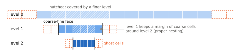
Some vocabulary:

A cell that is not covered by any finer cell is a leaf. The leaves, taken together over all levels, are the solution. The coarse cells under a fine patch still hold values (they're needed as boundary data and for refinement decisions), but they are not the answer.
A face where a patch ends is a coarse-fine face. One side of it is computed on a fine level and the other on a coarse one. Most of the difficulty of AMR lives at these faces.
Every patch has ghost cells beyond its ends, filled with boundary data before the patch is updated, exactly as a uniform grid has ghost cells for its boundary conditions. For a fine patch, "boundary data" means values interpolated from the coarser level.
Proper nesting means a patch on level $\ell+1$ lies strictly inside the level $\ell$ patches, with a margin of at least a cell or two. The reason: the fine patch's ghost cells must be fillable from genuine level $\ell$ data, not from level $\ell$'s own ghost cells.

Here is our data structure. I've made one simplification that production codes do not: each level stores a single array over the whole domain, plus a boolean mask own saying which cells it actually covers. That throws away the memory saving, which is half the point of AMR, but it keeps the code to a size you can read in one sitting. Real codes store only the patches and keep a list of them.

R = 2            # refinement ratio between levels
NG = 2           # ghost cells at each end of a level

class Level:
    def __init__(self, l, n0):
        self.l = l
        self.n = n0 * R**l
        self.h = (XMAX - XMIN) / self.n
        self.x = XMIN + (np.arange(self.n) + 0.5) * self.h
        self.u = np.zeros(self.n + 2 * NG)      # cell averages, ghosts included
        self.u_old = self.u.copy()              # state at the start of the current step
        self.own = np.zeros(self.n, bool)       # cells covered by this level
        self.F = np.zeros(self.n + 1)           # face fluxes from the last step
        self.Fsum = np.zeros(self.n + 1)        # dt-weighted fluxes summed over substeps

u_old, F and Fsum will each earn their keep later.

3. Moving data between levels

Two operations connect neighbouring levels, and both must respect the one thing finite-volume methods promise: the numbers are averages, and the total amount of stuff must not change when we copy them around.

Restriction goes fine to coarse. The coarse value under a fine patch is replaced by the average of the $R$ fine cells it contains. Since the fine cells have equal size, that's just their mean, and it conserves mass exactly.

def restrict(coarse, fine):
    """Overwrite coarse cells under the fine level with the fine averages."""
    under = fine.own.reshape(-1, R).all(axis=1)
    avg = fine.cells.reshape(-1, R).mean(axis=1)
    coarse.cells[under] = avg[under]
    return under

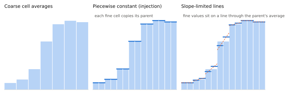
Prolongation goes coarse to fine, and it's where a choice has to be made. The simplest option, injection, gives every fine cell its parent's value. It conserves mass, but it turns a smooth coarse profile into a staircase, and if you do that at the boundary of a fine patch every time step you are feeding the fine grid a staircase as boundary data.

The better option reconstructs a line inside each coarse cell, exactly as in the reconstruction post, and reads the fine values off the line. Because the line passes through the cell average at the cell centre, the fine values average back to the coarse one, so mass is still conserved. And because the slope is limited (minmod here), the fine values never overshoot the neighbouring coarse values, so prolongation can't create a new peak or a negative density.

Prolongation, the coarse-to-fine step. Injection (middle) copies the parent value and makes a staircase. Slope-limited interpolation (right) places the two fine values on a line through the parent's average (dashed), so the average is preserved and the profile stays smooth. Where the profile flattens, the limiter reduces the slope to zero and the two coincide.

def prolong(uc):
    """Interpolate a coarse array (ghosts included) onto the fine cells under it."""
    s = np.zeros_like(uc)
    s[1:-1] = minmod(uc[1:-1] - uc[:-2], uc[2:] - uc[1:-1])
    offs = (np.arange(R) + 0.5) / R - 0.5
    fine = (uc[:, None] + s[:, None] * offs).ravel()
    start = NG * R - NG
    return fine[start:start + (len(uc) - 2 * NG) * R + 2 * NG]

(The last two lines just line the result up with the fine level's array, ghosts included.)

Prolongation is used for two different jobs: filling a fine patch's ghost cells every step, and giving newly refined cells their first values when the mesh changes. The same function does both.

4. Filling ghost cells, in space and in time

Before we update a level, every cell it will read must hold a sensible value. The cells it owns do. The others, its ghost cells and (in our whole-domain layout) everything outside its patches, need to be filled. On level 0 that's the physical boundary condition. On any finer level it's prolongation from the level below.

There's a subtlety that's easy to miss. We are going to take two fine steps for every coarse step (next section). The second fine step starts halfway through the coarse step, at $t + \Delta t/2$, and its ghost cells should hold the coarse solution at that time. The coarse level has no such thing; it jumped from $t$ to $t + \Delta t$. So we keep the coarse state from the start of the step (u_old) and interpolate linearly in time between it and the new state. That is what frac does:

def fill_ghosts(lv, coarse, frac):
    """Give every cell the level doesn't own a value."""
    if coarse is None:                      # base level: outflow boundaries
        lv.u[:NG] = lv.u[NG]
        lv.u[-NG:] = lv.u[-NG - 1]
        return
    uc = (1 - frac) * coarse.u_old + frac * coarse.u
    need = np.ones(lv.n + 2 * NG, bool)
    need[NG:-NG] = ~lv.own
    lv.u[need] = prolong(uc)[need]

Skipping the time interpolation is a classic bug. The simulation still runs, but fine patches see boundary data that is half a step stale, and waves passing through the coarse-fine face pick up errors and partial reflections.

5. Advancing in time: subcycling

A fine cell is $R$ times smaller than a coarse one, so the CFL condition gives it a time step $R$ times shorter. We could step the whole hierarchy at the finest level's $\Delta t$, which is simple and correct, but it wastes most of the saving: the coarse cells, which are the majority, would take $R^{\ell}$ times more steps than they need.

Instead, each level takes its own time step, and the schedule is recursive. This is the Berger–Oliger time stepping:

Advance level $\ell$ by $\Delta t_\ell$.
Advance level $\ell+1$ by $R$ steps of $\Delta t_\ell / R$, each of which recursively does the same for level $\ell+2$, and so on.
When level $\ell+1$ catches up with level $\ell$, synchronize: restrict the fine solution onto the coarse cells under it, and fix the fluxes at the coarse-fine faces (next section).

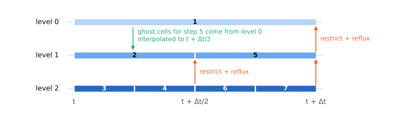
The order of operations for one coarse step with three levels and refinement ratio 2. The coarse level always goes first, so that the finer level has coarse data on both sides in time for its ghost cells. Each time a fine level catches up with its parent, the two are synchronized.

In code, it's a short recursive function. Note the order: the level is advanced before its children, and the children's results are folded back in afterwards.

def advance(levels, l, dt, frac=0.0, do_reflux=True):
    """Advance level l by dt, then every finer level by R substeps each."""
    lv = levels[l]
    fill_ghosts(lv, levels[l - 1] if l > 0 else None, frac)
    lv.u_old[:] = lv.u
    step(lv, dt)
    if l + 1 < len(levels):
        fine = levels[l + 1]
        fine.Fsum[:] = 0.0
        for k in range(R):
            advance(levels, l + 1, dt / R, k / R, do_reflux)
        under = restrict(lv, fine)
        if do_reflux:
            reflux(lv, fine, under, dt)

step is the uniform-grid Godunov update, applied to the cells the level owns. It also keeps the face fluxes, and adds them, weighted by $\Delta t$, to a running sum. Hold that thought.

def step(lv, dt):
    """One first-order Godunov step on the cells the level owns."""
    u = lv.u
    lv.F = riemann(u[NG - 1:NG + lv.n], u[NG:NG + lv.n + 1])
    lv.Fsum += dt * lv.F
    du = -dt / lv.h * (lv.F[1:] - lv.F[:-1])
    lv.cells[lv.own] += du[lv.own]

Notice that the coarse cells under a fine patch are updated too. That costs a little, but their fluxes are needed: the coarse flux through a coarse-fine face is computed as part of the coarse step, and it is about to matter a great deal.

6. Refluxing

Here is the problem. Look at a coarse-fine face. The coarse cell on its left was updated using the coarse flux $F_c$ through that face. The fine cells on its right were updated, over two substeps, using fine fluxes $F_f^1$ and $F_f^2$ through the same face. There is no reason for $F_c$ to equal the average of $F_f^1$ and $F_f^2$: they were computed from different data at different times.

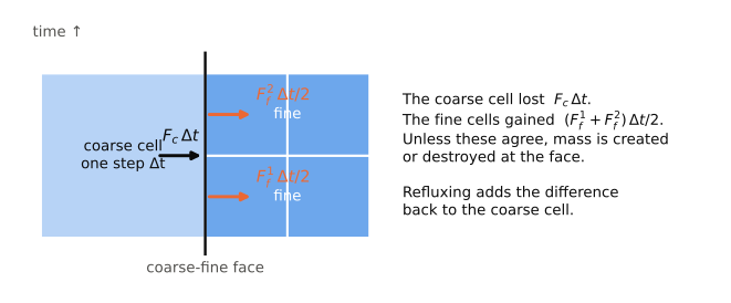
Why refluxing is needed. Both sides of a coarse-fine face must agree on what passed through it during the step; otherwise the finite-volume bookkeeping has a leak.

So what left the coarse cell is not what entered the fine cells, and mass has been created or destroyed at the face. The amounts are small per step, but they're systematic, and a shock sitting at a refinement boundary can leak mass at every step for the whole run.

The fix, called refluxing, is bookkeeping. We trust the fine fluxes, because they were computed on the better grid. So after the fine level catches up, we go back to the coarse cell and replace the coarse flux it used by the time average of the fine fluxes:

$$ u_c \;\mathrel{+}=\; \frac{\Delta t}{h_c}\left(F_c - \frac{1}{R}\sum_{k=1}^{R} F_f^{\,k}\right) $$

for the coarse cell on the left of a face where a fine patch begins, and the same with the opposite sign for the coarse cell on the right of a face where one ends. This is why step keeps F and accumulates Fsum: the coarse F is the flux we're correcting, and the fine Fsum is the sum we're correcting it with.

def reflux(coarse, fine, under, dt):
    """Make both sides of every coarse-fine face agree on the flux through it."""
    Feff = fine.Fsum[::R] / dt
    dF = dt / coarse.h * (coarse.F - Feff)
    starts = np.flatnonzero(under[1:] & ~under[:-1]) + 1   # faces where a fine region begins
    ends = np.flatnonzero(under[:-1] & ~under[1:]) + 1     # faces where one ends
    coarse.cells[starts - 1] += dF[starts]
    coarse.cells[ends] -= dF[ends]

After restriction and refluxing, every face in the hierarchy has a single flux that both of its neighbours used, and the total mass over the leaf cells is conserved to roundoff. Here's the measured mass error over the run with and without that correction. (The error is measured after accounting for the small amount of mass that flows out through the ends of the domain.)

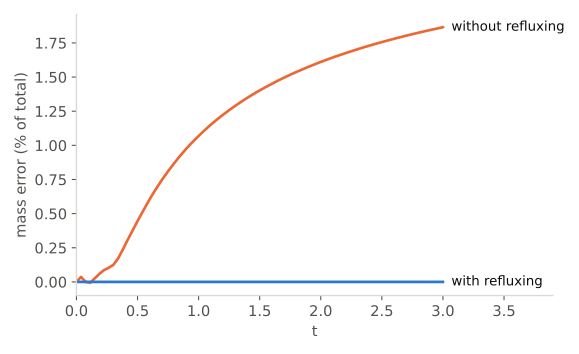
Mass error in percent of the total against time. Without refluxing the error grows to nearly two percent by t = 3, rising fastest when the shock forms. With refluxing the line stays at zero. — Total mass over the leaf cells, relative to the initial mass, with and without refluxing. The same code, with the one correction switched off, loses almost two percent of its mass in three time units. With it, the error is at the level of floating-point roundoff ($10^{-17}$).

Two percent might not sound like much. In a supernova simulation a few percent of the mass is the difference between a neutron star and a black hole, and in a cosmological simulation the error compounds over thousands of steps.

7. Deciding where to refine

Everything so far assumed we already know where the fine patches go. Now we let the solution decide. This happens in three stages: flag individual cells, buffer the flags, and cluster them into patches.

Flagging

A flag is a yes/no decision per cell: does this cell need to be finer? There are three broad families of criterion.

Look at the solution. Flag cells where the solution changes rapidly: a large jump to a neighbour, or a large second derivative. The most common version in astrophysics is the Löhner estimator (from Rainald Löhner's 1987 work on finite elements), which FLASH uses by default. It is a normalized second derivative,

$$ E_i = \frac{|u_{i+1} - 2u_i + u_{i-1}|}{|u_{i+1} - u_i| + |u_i - u_{i-1}| + \epsilon\,(|u_{i+1}| + 2|u_i| + |u_{i-1}|)}, $$

which lies between 0 and 1 and doesn't care about the units of $u$. Its weakness is that a smooth, large-scale feature on a coarse grid can look just as "curved" as a shock.

Estimate the error. Richardson's idea from 1911: solve the same problem at two resolutions and compare. In practice, coarsen the current solution by one level, interpolate it back, and look at the difference. Where the difference is large, the grid isn't resolving the solution. Berger and Oliger's original paper used a version of this, stepping the coarsened solution forward and comparing the result.

Use the physics. Astrophysics codes rarely rely on the generic estimators alone. They refine where the physics says resolution is needed, regardless of how smooth the solution looks: enough cells per Jeans length in a collapsing cloud, a minimum number of cells across a shock front, a maximum mass per cell in cosmology, a fixed resolution within some radius of a black hole or a sink particle.

Four stacked panels over x. Top: the Burgers' solution at t = 1.2, a ramp rising to about 0.7 and then dropping sharply to zero at the shock. Below it, three criteria: the jump to a neighbour, the Löhner estimator, and the difference from a coarsened copy. Each has a dashed threshold line and the cells above threshold are shaded. All three fire at the shock. The Löhner estimator also rises where the ramp bends into the flat region ahead of the shock. — Three refinement criteria applied to the same solution. All of them catch the shock. The Löhner estimator also responds to the smeared tail just ahead of the shock and to the foot of the ramp, which is the normalization at work: a small second derivative divided by an equally small first derivative. Whether those regions deserve refinement is a judgement call, and that's the point: a flagging criterion encodes what you think matters.

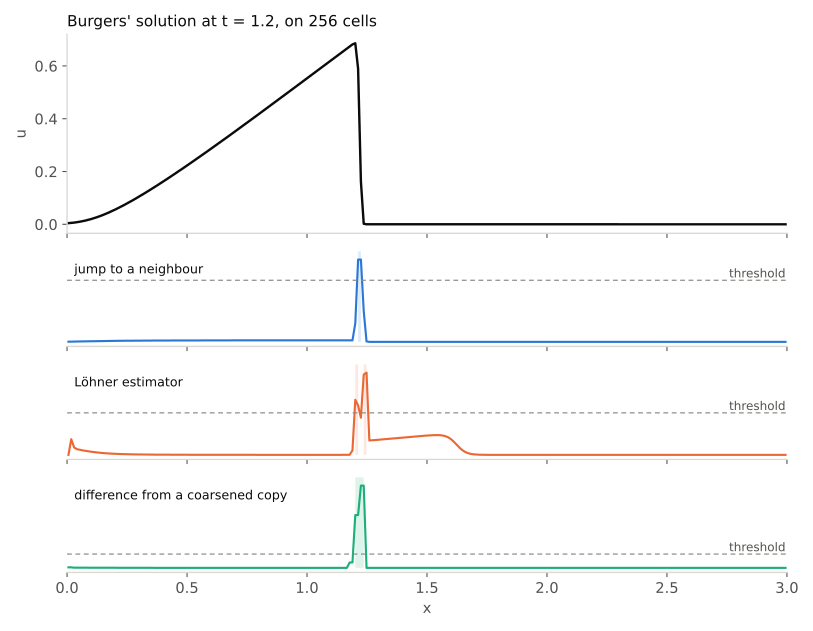
Our code uses the first criterion in its simplest form:

TOL = 0.08       # flag a cell when the jump to a neighbour exceeds this

def flag(lv):
    """Cells whose jump to either neighbour is larger than TOL."""
    u = lv.u
    jump = np.maximum(abs(u[NG + 1:NG + lv.n + 1] - u[NG:NG + lv.n]),
                      abs(u[NG:NG + lv.n] - u[NG - 1:NG + lv.n - 1]))
    return (jump > TOL) & lv.own

Notice that this criterion is applied on each level in turn, to that level's own data. Level 1 is built from the flags on level 0, level 2 from the flags on level 1, and so on. On the finer levels the same threshold is harder to trip, because the jump between neighbouring cells shrinks as the cells shrink, unless there is a shock, where it doesn't. That's exactly the behaviour we want: smooth regions stop being refined after a level or two, and shocks get refined all the way down.

Buffering

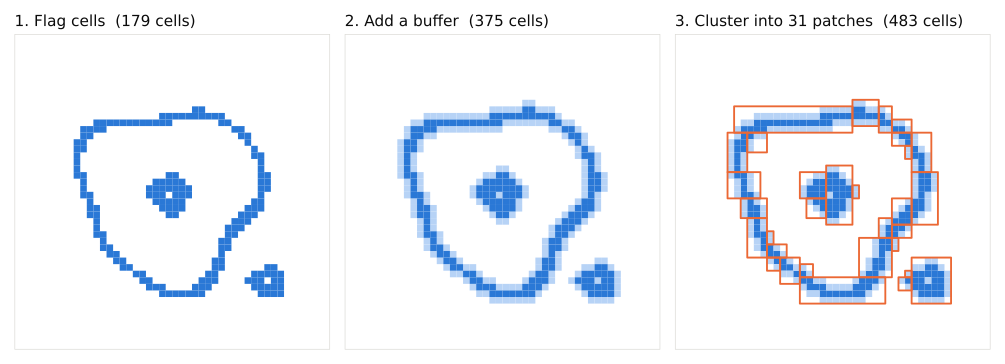
A fine patch that just barely covers the shock is a problem, because the shock moves. Between one regridding and the next it travels up to a cell per step, and if it crosses into the coarse region before we regrid, we've lost the resolution exactly where we wanted it. So every flag is buffered: the cells around it are flagged too, by a margin big enough to cover the motion until the next regrid.

Clustering

In one dimension, flagged cells group themselves into runs, and each run is a patch. In two and three dimensions it's a real problem: a thin curved shock front flags a thin curved band of cells, and we have to cover that band with rectangular boxes. Big boxes are cheap to manage but waste cells on unflagged regions; tiny boxes fit tightly but each one carries ghost cells and overhead.

The standard algorithm is Berger–Rigoutsos (1991). Take the bounding box of all flagged cells. Compute its signatures: the number of flagged cells in each row and each column. If the box is efficient enough (say, 70% of its cells are flagged), accept it. Otherwise look for a row or column with no flagged cells at all and split there; if there isn't one, split where the second derivative of the signature changes sign, which is where an edge of the flagged region is. Recurse on both halves.

Three panels of a 48 by 48 grid. Left: cells flagged along a lumpy ring (a shock front), around a central blob and around a small blob at lower right, 179 cells in all. Middle: the same with a one-cell buffer added in lighter blue, 375 cells. Right: 31 orange rectangles covering the buffered cells, 483 cells in total. — Flagging, buffering and clustering in two dimensions, for a shock front, a dense core and a small clump. The Berger–Rigoutsos algorithm covers the 375 buffered cells with 31 boxes containing 483 cells: an efficiency of 78%. Block-based codes skip this step by refining whole fixed-size blocks instead; tree codes skip it by refining single cells.

Regridding

Putting the stages together, regridding level $\ell+1$ means: flag on level $\ell$, buffer, restrict the flags to the properly nested region, and turn them into patches. Cells that were already refined keep their values. Cells that are newly refined get prolonged values from the coarse level. Cells that are no longer refined just disappear, and the coarse cells underneath, which were restricted at the last synchronization, carry on.

NEST = 2         # a refined cell must be this many coarse cells inside its parent level
NBUF = 2         # buffer cells added around flagged cells

def regrid(levels, l):
    """Rebuild level l+1 from the flags on level l."""
    coarse, fine = levels[l], levels[l + 1]
    allowed = ~dilate(~coarse.own, NEST)             # proper nesting
    want = dilate(flag(coarse), NBUF) & allowed
    fill_ghosts(fine, coarse, 1.0)                   # new cells get interpolated data
    fine.own = np.repeat(want, R)

dilate widens a mask by k cells on each side. Dilating the complement of the coarse level's coverage and taking the complement again shrinks the coverage by NEST cells, which gives the properly nested region.

We regrid after every coarse step, from the coarsest level up. Production codes regrid less often, every few steps, with a bigger buffer to compensate, since regridding in 3D with thousands of patches is expensive.

8. Putting it together

The driver sets up the base level, builds the initial hierarchy by regridding each level in turn, and then loops: pick the time step from the CFL condition, advance the whole hierarchy, regrid.

def run(u0, n0=64, lmax=3, T=3.0):
    levels = [Level(l, n0) for l in range(lmax + 1)]
    base = levels[0]
    base.own[:] = True
    base.cells[:] = u0(base.x)
    fill_ghosts(base, None, 0.0)
    for l in range(lmax):
        regrid(levels, l)
    t = 0.0
    while t < T:
        umax = max(abs(lv.cells[lv.own]).max() for lv in levels if lv.own.any())
        dt = min(CFL * base.h / umax, T - t)
        advance(levels, 0, dt)
        t += dt
        for l in range(lmax):
            regrid(levels, l)
    return levels

With 64 base cells and three levels of refinement, the finest cells are $3/512$ wide. Here's what the solution and the hierarchy look like, compared with uniform grids of 64 and 512 cells.

Four panels at t = 0, 1, 2 and 3. Each shows the AMR solution in blue, a 64-cell uniform solution in orange and a 512-cell uniform solution dashed grey. Under each plot, horizontal bands show which level owns each part of the domain: level 0 almost everywhere, with levels 1, 2 and 3 nested around the shock, moving right with it. At t = 0 the refined region covers the bump; later it is a narrow stack of levels at the shock. The AMR curve lies on top of the fine uniform curve, while the 64-cell solution smears the shock over several cells. — The AMR run (blue) against uniform runs on 64 cells (orange) and 512 cells (dashed). The bands below each plot show the leaf cells of each level, light to dark from level 0 to level 3. The hierarchy follows the shock as it forms and moves. The AMR solution is indistinguishable from the 512-cell one at the shock, where it has the same resolution, and uses level 0 almost everywhere else.

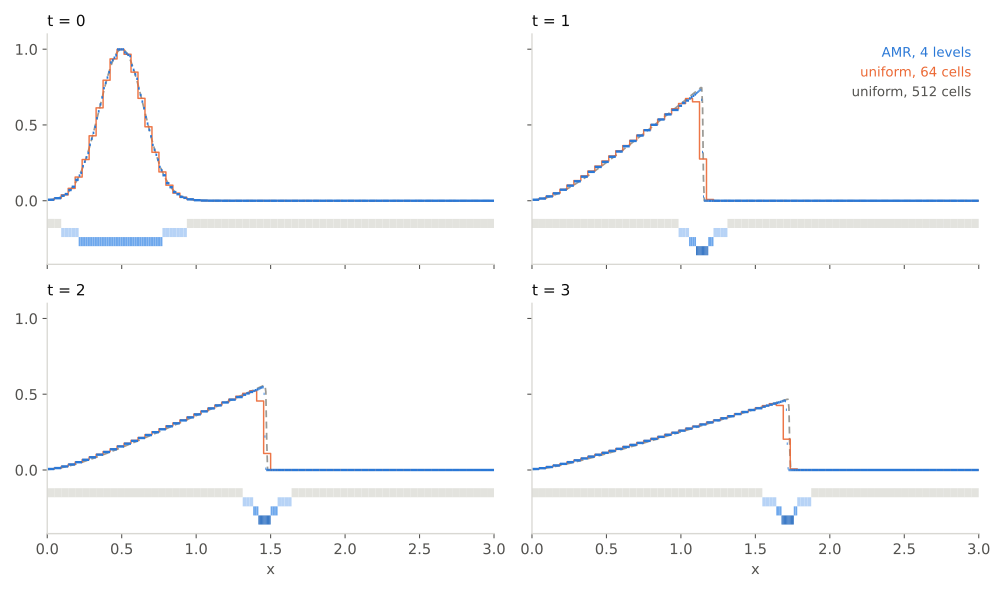
The numbers behind the picture: the AMR run performs about 15,000 cell updates. The uniform 512-cell run, which is what you'd need to get the same shock, performs 226,000. That's a factor of 15, in one dimension, for a problem where the "interesting" region is already a decent fraction of the domain. In 3D, where a shock front is a surface in a volume, the factor is routinely in the hundreds or thousands.

Away from the shock the AMR solution is a 64-cell solution, and you can see it: the smooth ramp behind the shock is slightly more smeared than the 512-cell one. AMR gives you the resolution you asked for where you asked for it, and no more. If you care about the smooth part, flag the smooth part.

9. What changes in three dimensions

Everything above carries over to 3D unchanged in principle. Restriction averages $R^3$ cells instead of $R$. Prolongation uses limited slopes in each direction. Refluxing happens on the faces of boxes instead of at two points. The recursion in advance is identical. What's new is the engineering, and some physics that doesn't fit the pattern.

Organizing the cells. A 3D code has to keep track of thousands of boxes, their neighbours, which processor holds them, and where their coarse-fine faces are. Three designs are in use. Patch-based codes (Enzo, the AMReX family: CASTRO, MAESTROeX, Nyx) cluster flagged cells into boxes of arbitrary size, as above. Block-based codes (FLASH, Athena++) make every box the same size, say $16^3$ cells, and refine by replacing a block with eight children; there's no clustering step, and every block looks the same to the rest of the code, which makes it easy to run on GPUs. Tree-based codes (RAMSES) refine single cells into eight children, organized as an octree. The mesh fits the solution very tightly, at the cost of more pointer-chasing per cell.

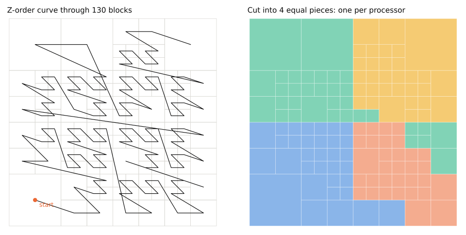
Load balancing. The work moves around as the mesh changes, and the boxes have to be redistributed among processors so that each has about the same number of cells and its neighbours are mostly on the same processor. The standard trick is to order the blocks along a space-filling curve, Morton (Z-order) or Hilbert, and cut the curve into equal pieces. Blocks that are close along the curve are close in space, so each processor gets a compact chunk.

Left: a two-dimensional quadtree mesh with 130 blocks of different sizes, with a Z-order curve threading through every block in order, starting at the lower left. Right: the same blocks coloured in four colours, one per processor, by cutting the curve into four equal pieces. Each colour forms a mostly compact region. — Load balancing with a space-filling curve. The Z-order (Morton) curve visits every block once, and nearby blocks are mostly nearby on the curve. Cutting the curve into four equal pieces gives four processors compact regions with roughly equal work. The Hilbert curve does the same with fewer long jumps.

Gravity. Self-gravity means solving Poisson's equation, an elliptic problem where every cell talks to every other. On a hierarchy, that's done with multigrid methods that pass corrections up and down the levels, and the potential at a coarse-fine face has to be matched carefully or the gravitational force is discontinuous there, which then shows up as spurious accelerations. In our 1D code, conservation of mass came from refluxing. With gravity, total energy isn't exactly conserved on an adaptive mesh even with refluxing, because the potential changes when the mesh changes; codes track this and report it.

Magnetic fields. The magnetic field must satisfy $\nabla \cdot \mathbf{B} = 0$. MHD codes keep it that way with constrained transport, which stores the field on cell faces rather than cell centres. Prolongation and restriction of a face-centred field have to preserve the zero divergence, and ordinary interpolation does not. Dinshaw Balsara's 2001 divergence-free prolongation is the standard solution, and every AMR MHD code has some version of it.

Particles. Cosmological simulations carry dark matter as particles that move through the mesh. Each particle lives on the finest level that covers its position, deposits mass onto that level for the gravity solve, and reads the force back. Star and sink particles work the same way. When the mesh changes under a particle, it has to be handed from one level's list to another's.

Physics that doesn't subcycle well. Berger–Oliger time stepping assumes the physics on each level is local and explicit. Radiation transport, chemistry with stiff reaction networks, and implicit diffusion often aren't. Codes either step those parts of the physics at the coarse time step for all levels, or solve them on the whole hierarchy at once with an implicit solver.

10. The things that go wrong

A few failure modes are worth knowing about, because they're common and hard to spot:

Reflections at refinement boundaries. A fine grid can carry waves the coarse grid can't. When such a wave reaches a coarse-fine face, part of it reflects. In a turbulence simulation, this means the refinement boundary itself becomes a source of spurious motion. Deeper buffers and gentler jumps in resolution (ratio 2, not 4) help.
Resolution-dependent physics. A refinement criterion that changes the resolution also changes the numerical viscosity. Turbulence, mixing instabilities and magnetic dynamos all depend on the resolution they're given. Refining only around shocks can mean the turbulence behind the shock is underresolved in a way that is hard to see.
The criterion encodes your expectations. If you flag on density gradients, you'll resolve shocks. If you flag on Jeans length, you'll resolve collapse. Something unexpected, a weak instability growing slowly in a smooth region, say, may never trigger refinement and never be seen. The honest check is to change the criterion, or the thresholds, and see whether the result changes.
Refining at the right time. A fine patch that appears after a shock has formed on the coarse grid inherits a smeared shock. The interpolated profile is then advected at the fine resolution, and the shock stays wider than it should. The buffer and regrid interval are tuned to refine before structure forms, not after.
Cost. AMR is only cheaper if the refined region is a small fraction of the volume. A simulation of fully developed turbulence, where every cell needs resolution, gains nothing from AMR and pays the overhead. Know your problem.

Exercises

If you want to make the ideas stick, the script is short enough to experiment with.

Switch off the time interpolation by replacing frac with 1.0 in advance. Watch what happens at the coarse-fine faces, especially while the shock forms.
Use injection instead of limited slopes in prolong. Compare the results away from the shock.
Change the refinement ratio to 4. You'll need to check that every place R appears still makes sense, and that NEST and NBUF are large enough.
Make the scheme second order with minmod or MC reconstruction and a two-stage Runge–Kutta step. The ghost cell count NG is 2 for a reason. What changes in reflux when the time stepping has more than one stage?
Flag on the Löhner estimator instead of the jump, and compare the hierarchies.
Move to a system. Replace Burgers' equation with the Euler equations and the HLLC flux from the reconstruction post. Mass, momentum and energy all need refluxing now, and you'll have to decide what to flag on.