The curse of dimensionality, and how astrophysics codes cheat it

The last two posts were about what to compute in each cell of a simulation. This one is about something that matters even more in practice: where to put the cells. In astrophysics, that question is often what decides whether a simulation can be done at all.

A factor of a billion

Take the death of a massive star. When the iron core collapses, it forms a proto-neutron star a few tens of kilometres across. Neutrinos pour out of it and the shock wave stalls above it. To follow the neutrinos and the turbulent flow there, you need grid cells around half a kilometre across. Meanwhile, the star's outer layers extend to hundreds of millions of kilometres. If you want to follow the explosion all the way out, or simply know how much mass will fall back onto the neutron star, all of that is in the problem too.

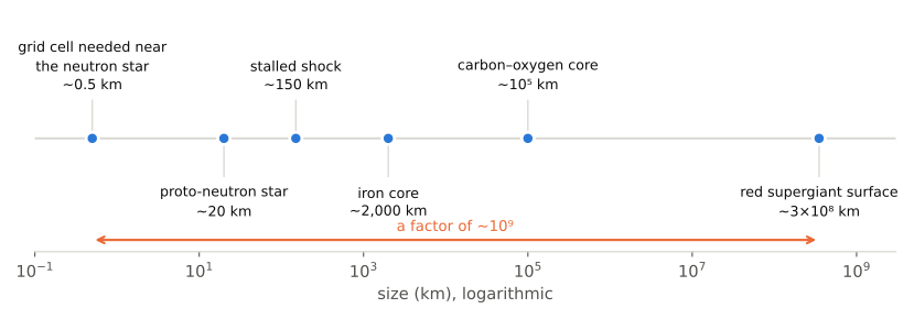
Cover that range with a uniform grid of half-kilometre cells and you need about a billion cells along each side. In three dimensions that is \(10^{27}\) cells, more than the number of grains of sand on Earth, many times over. No computer will ever store that.

The other places astrophysicists look are no better. A cosmological simulation needs a box hundreds of millions of light years across to get a fair sample of the universe, but stars form in clouds a few light years across. An accretion disk around a black hole needs resolution near the horizon, a few kilometres, and also has to reach out to where the disk is fed, thousands of times further.

Why three dimensions is so much worse than one

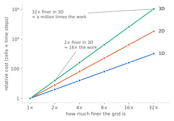
The phrase curse of dimensionality comes from Richard Bellman, who was writing about optimization in 1957, but it fits grids perfectly. Suppose you make a grid \(k\) times finer:

• In 1D you have \(k\) times as many cells. In 3D you have \(k^3\) times as many.
• Because of the CFL condition (see the last post), smaller cells force smaller time steps, so you also need \(k\) times as many steps.

The total work grows like \(k^{d+1}\) in \(d\) dimensions. Doubling the resolution of a 3D simulation costs \(2^4 = 16\) times as much. Going 32 times finer, which is still nowhere near a factor of a billion, costs a million times as much.

Memory is a hard limit too. A grid of \(1000^3\) cells, with ten numbers per cell for density, velocity, energy, magnetic field and composition, already takes 80 GB, and real codes store several copies of everything.

The oldest trick: use fewer dimensions

For decades, the main way out was symmetry. If a star is assumed to be spherical, it is a 1D problem, and you can afford thousands of radial zones and very detailed physics. If it is assumed to be symmetric about an axis, it is 2D. Most supernova modelling before about 2015 was done this way, and much of it still is.

The catch is that the symmetry is never real, and in some problems it changes the answer. Supernova explosions are driven by turbulent convection and a sloshing instability of the shock, and turbulence in 2D behaves differently from 3D. In 2D, energy tends to move from small swirls into big ones; in 3D it cascades the other way. So 2D models can explode when the 3D version doesn't, or the other way round. The field has spent the last decade working out which 2D results survive in 3D. Every method below is a way to make full 3D affordable.

Coordinates that fit the problem

The cheapest improvement is to choose coordinates that match the shape of the problem. A star is roughly spherical, so use spherical coordinates and space the radial shells logarithmically: each shell is a fixed percentage thicker than the one inside it. Cells are then about half a kilometre wide near the neutron star and thousands of kilometres wide in the envelope. Twenty shells per factor of ten in radius covers a factor of a billion in fewer than 200 shells. HARM-type codes for black-hole accretion do the same thing, with radial spacing that grows outwards and angular cells packed towards the disk midplane.

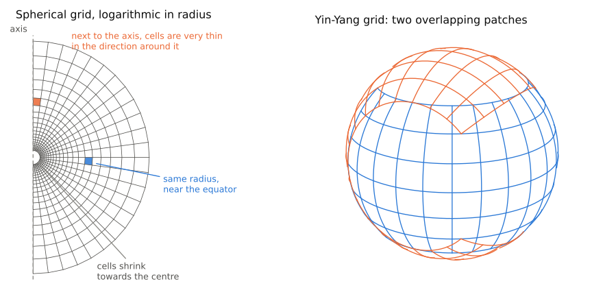
Spherical grids bring their own problems, both at singular points of the coordinates:

• The pole. In a latitude–longitude grid, cells near the axis are very thin in the direction around it. The CFL condition is set by the smallest cell, so a handful of cells near the poles can force the whole simulation to take tiny time steps. Fixes include merging cells near the poles (the "dendritic" grid of the Fornax supernova code), the Yin-Yang grid (Kageyama and Sato, 2004), used in 3D supernova simulations with PROMETHEUS-HOTB, or a cubed sphere, which projects the six faces of a cube onto the sphere.
• The centre. All the radial lines meet at \(r = 0\). Codes either cut the centre out and replace it with a boundary condition, use a small Cartesian patch there, or simply leave out the inner core and model the neutron star as a boundary.

Nested grids

The next idea is the most literal one: put a finer grid inside the coarse grid, wherever the action is. Each level is a box half the size of the previous one with the same number of cells, so its cells are half the size. Five levels gain a factor of 16 in resolution. Twenty levels gain a factor of about a million, and each level costs the same as the coarsest.

These nested (or "static mesh refinement") grids are the workhorse of numerical relativity. The Carpet framework (Schnetter, Hawley and Hawke, 2004) and its descendants put nested boxes around each black hole or neutron star in a merging binary, and move the boxes along with the objects as they orbit. The 2005 breakthroughs in simulating merging black holes used mesh refinement of this kind, and their descendants helped calibrate the waveform models LIGO uses. Several 3D general-relativistic supernova codes also use nested Cartesian boxes centred on the collapsing core.

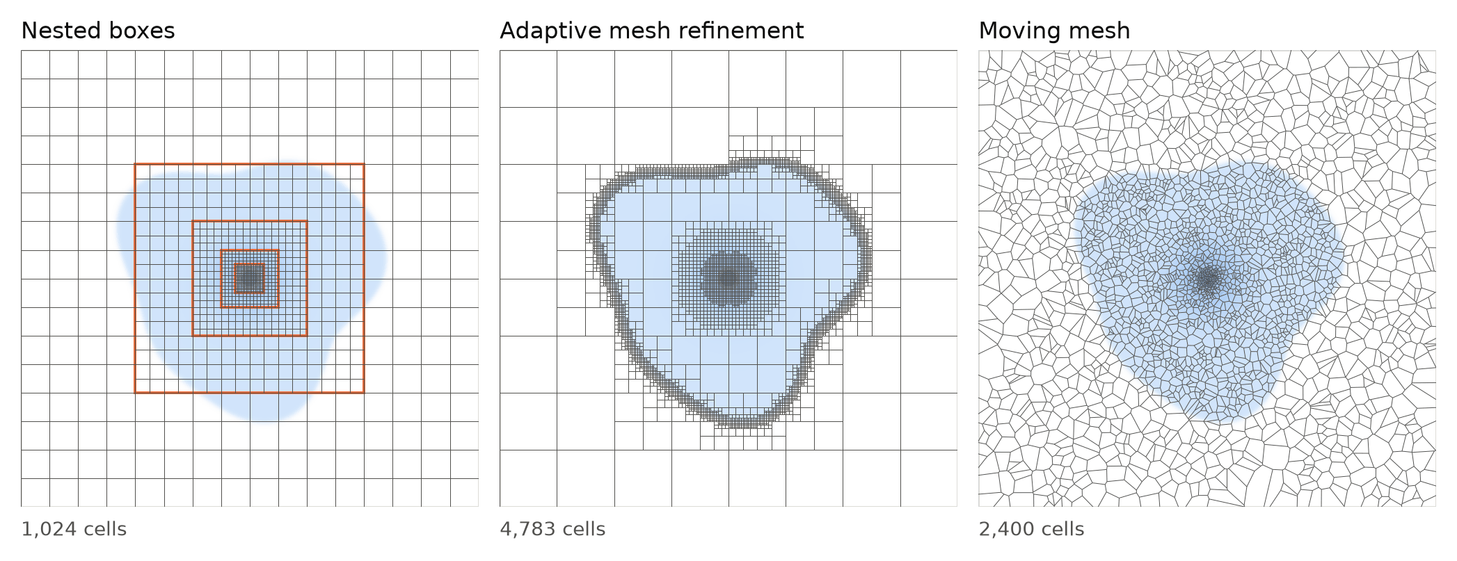
Benefits. Nested grids are simple and predictable. Every level is a regular grid, so the fast, accurate methods from the previous posts work unchanged inside it. The memory use is known in advance, and it is easy to split the work evenly across processors.

Challenges. The interfaces between levels are where most of the trouble is:

• Reflections. A wave leaving a fine grid for a coarse one suddenly finds itself under-resolved. Short waves that the coarse grid can't represent can partly reflect off the interface, back into the region you care about.
• Time steps. Fine levels need smaller time steps. Instead of stepping everything at the finest rate, codes subcycle: each fine level takes two steps for every one of its parent. Values at the boundary of the fine grid then have to be interpolated in time from the coarse grid.
• Conservation. The coarse cell next to an interface and the fine cells on the other side compute slightly different fluxes through the same face. To keep mass and energy exactly conserved, codes go back and correct the coarse cell with the fine fluxes (refluxing).
• You have to know in advance. The boxes sit where you put them. A shock that leaves the fine box, or a structure that forms somewhere unexpected, is simply under-resolved.

Adaptive mesh refinement

The last point is the big one, and the answer is to let the simulation decide. Adaptive mesh refinement (AMR) checks the solution as it evolves, flags the cells that need more resolution, and covers them with finer grids. Grids are added and removed as features move. The method was developed by Marsha Berger with Joseph Oliger (1984) and Phillip Colella (1989), and it has spread through most of computational astrophysics.

There are three main ways to organize the refined cells:

• Patch-based AMR covers flagged regions with rectangular patches of any size, as in Berger and Colella's original work. Enzo works this way, as do the codes built on the AMReX library, such as CASTRO and MAESTROeX for stellar explosions and convection.
• Block-based AMR splits the domain into blocks of a fixed size, say \(16^3\) cells, and refines a whole block by replacing it with eight children. FLASH (through PARAMESH) and Athena++ work this way. Fixed-size blocks are easy to distribute across thousands of processors.
• Tree-based AMR refines individual cells, each splitting into eight children in an octree. RAMSES (Teyssier, 2002), widely used in cosmology and galaxy formation, works this way.

What to refine on. This is where the physics comes in. Common choices:

• Steep gradients, or an estimate of the local error, such as the Löhner estimator used in FLASH, which picks up shocks and fronts.
• Enough cells per Jeans length, in star formation. Truelove and collaborators showed in 1997 that if a collapsing gas cloud has fewer than about four cells per Jeans length, the scale on which gravity overcomes pressure, it breaks up into spurious fragments.
• A fixed mass per cell, in cosmology, so that resolution follows the matter as it collapses into galaxies.

Benefits. AMR puts resolution where the solution needs it, even when you can't predict where that will be, and it keeps the accuracy of regular grids inside each patch. It routinely spans factors of \(10^6\) or more in scale. Simulations of the first stars (Abel, Bryan and Norman, 2002) followed a collapsing gas cloud over a range of more than \(10^{10}\) in length this way.

Challenges. All the interface problems of nested grids are still there, and there are more of them, and they move:

• Bookkeeping. Every level needs ghost cells filled by interpolating from coarser levels (prolongation) and averaging from finer ones (restriction), plus refluxing and subcycling, all done in a way that stays conservative and doesn't create new oscillations. For magnetic fields, interpolation must also keep \(\nabla \cdot \mathbf{B} = 0\), which needs special schemes (Balsara, 2001).
• Gravity. Solving for the gravitational field on a hierarchy of grids needs multigrid-style solvers that stitch the levels together.
• Load balancing. As the mesh changes, the work moves around. Codes regularly redistribute blocks among processors, often by ordering them along a space-filling curve (Morton or Hilbert), so that each processor gets a compact chunk of space.
• The criterion is a physics choice. AMR resolves what you told it to look for. A refinement criterion tuned for shocks may completely miss the slow growth of a turbulent instability, and turbulence near a refinement boundary sees an abrupt change in numerical viscosity.
• Complexity. An AMR framework is a large piece of software, and irregular data structures are a poor fit for GPUs. This is one reason newer frameworks such as AMReX and Parthenon keep their blocks large and regular.

Let the mesh move with the gas

A completely different approach is to let resolution follow the mass automatically by making the computational elements move with the flow.

Smoothed particle hydrodynamics (SPH, 1977, independently by Lucy and by Gingold and Monaghan) does away with the grid entirely. The gas is a collection of particles, each carrying a fixed mass. Where gas collects, particles collect, and resolution increases with no refinement logic at all. SPH ran most of the cosmological and star-formation simulations of the 1990s and 2000s, and it is still standard for neutron-star mergers in some groups and for planetary collisions.

Moving-mesh codes combine the two ideas. AREPO (Springel, 2010) builds a Voronoi mesh around points that move with the gas, and solves the finite-volume equations from the previous posts on its constantly changing, irregular cells. It ran the Illustris and IllustrisTNG cosmological simulations. Meshless methods such as GIZMO (Hopkins, 2015) solve Riemann problems between neighbouring particles without building cells at all.

Benefits. Resolution follows the mass for free. Material moving quickly across the domain, such as a galaxy in a cluster or a disk orbiting a star, doesn't suffer the numerical diffusion that comes from being carried through a fixed grid. And there is no refinement criterion to get wrong.

Challenges.

• Mass isn't always where the physics is. A shock running into thin gas, a hot, diffuse outflow or the low-density funnel above a black hole all have few particles and therefore poor resolution, even if they are the interesting part.
• Classic SPH struggled with mixing. A well-known comparison by Agertz and collaborators (2007) showed that standard SPH suppresses the instabilities that mix gas layers moving past each other, which grid codes capture. Modern SPH variants largely fix this, but it was a large part of why moving-mesh and meshless methods were developed.
• Keeping the mesh tidy. A moving mesh gets tangled in shearing flows, so the codes nudge the points to keep the cells well shaped, at the cost of some of the purely Lagrangian behaviour.

Other ways to cheat

A few more tricks are in everyday use:

• Zoom-in simulations. In cosmology, run a coarse simulation of a big box, pick one galaxy, trace its matter back to the early universe, and rerun with high resolution only in that region and coarse particles everywhere else. Tools like MUSIC (Hahn and Abel, 2011) generate the initial conditions. Most detailed simulations of Milky Way–like galaxies are zoom-ins.
• Excision. Don't simulate what you don't need. Black-hole codes place their inner boundary inside the event horizon, where nothing can get back out, and many supernova simulations replace the inner neutron star with a boundary condition.
• Subgrid models. When you can't resolve something, model it. Sink particles (Bate, Bonnell and Price, 1995; Krumholz, McKee and Klein, 2004) replace a collapsing protostar with a point mass that accretes gas, so that the simulation doesn't have to follow the collapse down to stellar sizes. Galaxy simulations use recipes for star formation and supernova feedback that act on scales far below a cell.
• Splitting the problem in time. Simulate the core collapse in detail for the first second or so, then map the result onto a coarser grid that follows the explosion as it moves out through the star for hours or days.

When the space isn't just space

The curse is at its worst in radiation and neutrino transport. To describe the neutrinos streaming out of a supernova core, you need to know how many are at each point in space (three dimensions), travelling in each direction (two more) with each energy (one more). That is a six-dimensional space plus time. Even a crude 100 points per dimension gives \(10^{12}\) unknowns per time step, before you count neutrino species.

Grid-based transport codes cope by being clever about the angles. The discrete ordinates method keeps a modest set of directions. Moment methods such as M1 keep only the first few averages over direction, and supply an approximate closure for the rest.

The other option is to stop using a grid in the extra dimensions. In Monte Carlo transport, you follow a large number of sample "packets" of neutrinos or photons. Each packet is emitted, flies, scatters and is absorbed according to random numbers drawn from the physical probabilities. The error of a Monte Carlo estimate shrinks like \(1/\sqrt{N}\) in the number of samples, no matter how many dimensions there are. On a grid with second-order accuracy, the error shrinks like \(N^{-2/d}\) in the number of points. Above four dimensions, Monte Carlo wins.

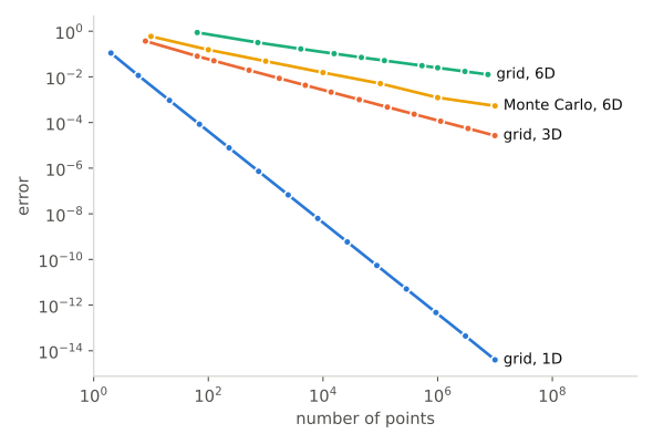
This is the approach in νbhlight, the code I use for collapsar disks. It couples general-relativistic MHD on a grid to Monte Carlo neutrino transport, so the fluid lives in three dimensions while the neutrinos sample the full phase space. Monte Carlo has costs of its own. The answers are noisy, so you need a lot of packets. And where matter is very dense, a packet scatters millions of times before it escapes, which is prohibitively expensive. Codes handle that with hybrid schemes that switch to a diffusion description in those regions.

In short

The curse of dimensionality is the reason astrophysical simulation is as much about where to compute as about what to compute:

Method	Resolution goes…	Main strength	Main headache
Symmetry (1D/2D)	everywhere, cheaply	affordable detail	the real thing is 3D
Stretched/spherical grids	where the geometry says	simple, very cheap	poles and the centre
Nested grids	where you put it	simple, regular, predictable	must know in advance
AMR	where the solution needs it	adapts to anything	complexity, level interfaces
Particles / moving mesh	where the mass is	no criterion needed, low diffusion	thin gas is poorly resolved
Monte Carlo (for transport)	to wherever packets go	error independent of dimension	noise, dense regions

In practice, production codes combine several of these. A modern supernova simulation might use a spherical grid with a special treatment near the pole, a moving inner boundary and a moment method for the neutrinos. A galaxy simulation might combine a zoom-in, AMR or a moving mesh, and subgrid models for star formation. The physics hasn't changed since Richardson's time. Choosing where to put the cells is what keeps getting cleverer.